![]()
home2park is an R package for assessing the spatial provision of urban parks to residential buildings city-wide. Refer to the package website for demonstrations of how the package may be used.
Installation
Install the development version of home2park from GitHub:
devtools::install_github("ecological-cities/home2park", ref = "main")Citation
To cite home2park or acknowledge its use, please cite the following:
Song, X. P., Chong, K. Y. (2021). home2park: An R package to assess the spatial provision of urban parks. Journal of Open Source Software, 6(65), 3609. https://doi.org/10.21105/joss.03609
The get a BibTex entry, run citation("home2park").
Background
Parks are important spaces for recreation and leisure in cities. Conventional measures of park provision tend to rely on summaries of park area within a given region (e.g. per capita park area). However, there is a need to characterise the wide variety of parks (e.g. nature areas, gardens, waterfront parks, outdoor playgrounds, etc.) that serve different groups of people. When planning at fine spatial scales, such current metrics are also limited by their coarse spatial resolution and the presence of artificial boundaries.
Using home2park
The package home2park provides a way to measure multiple aspects of park provision to homes, at the resolution of individual buildings. The key features include the ability to:
- Download relevant data from OpenStreetMap (OSM) such as buildings, parks and features related to recreation. The user may also supply data for new buildings and parks, for the purpose of future scenario planning.
- Redistribute coarse-scale population data per census unit into residential buildings, also known as ‘dasymetric mapping’, which helps highlight specific areas where more people will benefit from the presence of parks.
- Summarise at each park multiple attributes that are important for recreation (e.g. dense vegetation, length of waterfronts, open spaces, trails, etc.).
- Calculate the supply (provision) of the park attributes to each residential building, while accounting for ‘distance decay’, or the fact that supply from parks further away are reduced.
The following sections provide a high-level overview of the various steps required to measure the spatial provision of parks. Further details and code examples can be found in the package vignette ‘Get started’.
1. Process city population
Residential buildings (homes) are an important component of the analysis. These may be obtained, for example, by downloading building polygons from OpenStreetMap (OSM), and subsetting the dataset to areas within ‘residential’ land use zones.
In addition, having the population count per residential building allows us to calculate the total spatial provision of parks to all residents, and can help highlight important areas where more people will benefit from the presence of parks. Coarse-scale population census data can be redistributed into the residential buildings, via a technique known as ‘dasymetric mapping’. The number of building ‘levels’ from OSM can be used as a proxy for population density (i.e. more residents per unit area). Here’s an example screenshot showing an overlay of multiple example datasets in the package (for the city of Singapore), which were used to redistribute population data per census unit (subzones) across residential buildings.
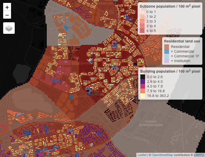
Example screenshot showing an overlay of multiple datasets used to redistribute the population across buildings within residential land use zones. The legends are ordered (top to bottom) by increasing spatial resolution.
Residential building polygons in Singapore each with a population count can be found in the following example dataset:
data(buildings_pop_sgp)
head(buildings_pop_sgp)
#> Simple feature collection with 6 features and 1 field
#> Geometry type: POLYGON
#> Dimension:     XY
#> Bounding box:  xmin: 103.8412 ymin: 1.297955 xmax: 103.8968 ymax: 1.426561
#> Geodetic CRS:  WGS 84
#>    popcount                       geometry
#> 1 32.367111 POLYGON ((103.8412 1.420676...
#> 2 20.880897 POLYGON ((103.8808 1.320019...
#> 3  2.311594 POLYGON ((103.8643 1.320283...
#> 4 56.747406 POLYGON ((103.8504 1.303723...
#> 5  6.368404 POLYGON ((103.8516 1.426561...
#> 6  9.502521 POLYGON ((103.8966 1.298226...
2. Process parks
Parks are the other important component of the analysis. These may be downloaded from OSM and processed using this package. The following example dataset contains parks in Singapore with selected attributes related to recreation/leisure:
data(parks_sgp)
head(parks_sgp[, 28:33]) # subset to relevant columns
#> Simple feature collection with 6 features and 6 fields
#> Geometry type: MULTIPOLYGON
#> Dimension:     XY
#> Bounding box:  xmin: 103.7809 ymin: 1.248586 xmax: 103.8704 ymax: 1.28586
#> Geodetic CRS:  WGS 84
#>               area     perimeter playground_count playground_ptdensity
#> 1   2454.365 [m^2]  346.5265 [m]                0            0 [1/m^2]
#> 2   1964.286 [m^2]  305.3844 [m]                0            0 [1/m^2]
#> 3 219319.203 [m^2] 3019.2241 [m]                0            0 [1/m^2]
#> 4  22513.834 [m^2]  615.1039 [m]                0            0 [1/m^2]
#> 5 571259.766 [m^2] 3973.5567 [m]                0            0 [1/m^2]
#> 6  67533.345 [m^2] 1092.2758 [m]                0            0 [1/m^2]
#>    trails_length trails_length_perim_ratio                       geometry
#> 1     0.0000 [m]             0.0000000 [1] MULTIPOLYGON (((103.8471 1....
#> 2     0.0000 [m]             0.0000000 [1] MULTIPOLYGON (((103.8446 1....
#> 3  4072.5481 [m]             1.3488724 [1] MULTIPOLYGON (((103.8059 1....
#> 4   837.9212 [m]             1.3622434 [1] MULTIPOLYGON (((103.8233 1....
#> 5 20947.6579 [m]             5.2717652 [1] MULTIPOLYGON (((103.8613 1....
#> 6   905.5080 [m]             0.8290105 [1] MULTIPOLYGON (((103.7812 1....
3. Recreation supply
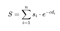
With the processed building and park polygons, the provision of park attributes per residential building can be calculated. The total supply S of each park attribute to a building is calculated based on the following equation. Its value depends on the distances between that particular building and all parks; attributes from parks further away are reduced as a result of the negative exponential function e-cd, an effect also known as the ‘distance decay’ (Rossi et al., 2015).
where
S = Total supply of a specific park attribute to the building from parks i; i = 1,2,3, … n where n = total number of parks citywide.
si = Supply of a specific park attribute from park i. A perfect positive linear association is assumed, since the focus is on supply metrics.
di = Distance in kilometres from the building to park i (e.g. Euclidean, Manhattan, etc.).
c = Coefficient determining rate of decay in supply si with increasing distance.
Note that the value of Coefficient c depends on both park and park visitors’ attributes, such as socio-demographic factors and preferences for activities that may impel shorter or longer travel (Rossi et al., 2015; Tu et al.). A lower value implies that parks further away are accessible or frequently visited by residents (i.e. still contributes to the ‘recreation supply’ of a particular building).
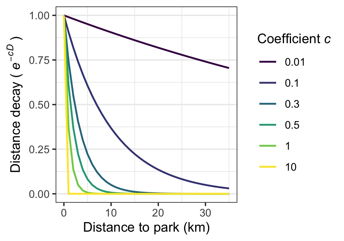
Figure: The value of Coefficient c and its effect on the distance decay between a building and park.
Screenshot: Examples showing the supply of OSM park area to residential buildings in Singapore for the year 2020 when the value of Coefficient c is 0.1 (left panel) and 1 (right panel). Each building is denoted as a point (a random subset is shown); the color palette is binned according to quantile values.
To calculate the supply of each park attribute, we first calculate the pairwise distances between all buildings and parks (a distance matrix). This output is supplied to the function recre_supply(). For example, we can calculate the supply of park area to each building. This supply value can then be multiplied by the population count per building, to obtain the total supply to all residents.
# transform buildings & parks to projected crs
buildings_pop_sgp <- sf::st_transform(buildings_pop_sgp, sf::st_crs(32648))
parks_sgp <- sf::st_transform(parks_sgp, sf::st_crs(32648))


# convert buildings to points (centroids), then calculate distances to every park
m_dist <- buildings_pop_sgp %>%
  sf::st_centroid() %>%
  sf::st_distance(parks_sgp) %>% # euclidean distance
    units::set_units(NULL)

m_dist <- m_dist / 1000 # convert distances to km


# new column for the supply of park area
buildings_pop_sgp$area_supply <- recre_supply(park_attribute = parks_sgp$area,
                                              dist_matrix = m_dist,
                                              c = 0.302) # e.g. from Tu et al. (2020)

# supply to all residents per building
buildings_pop_sgp$area_supplytopop <- buildings_pop_sgp$area_supply * buildings_pop_sgp$popcount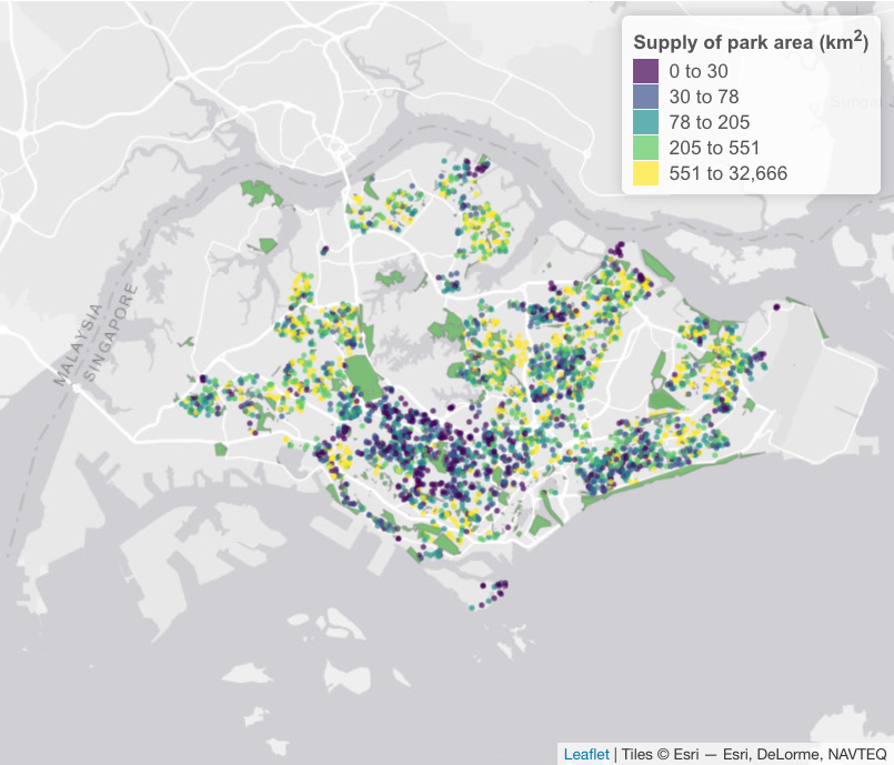
Screenshot: Supply of park area to building residents in Singapore based on OSM data (2020). Each building is denoted as a point (a random subset is shown). The value for Coefficient c was set at 0.302. The color palette is binned according to quantile values.
Data sources
Singapore census data from the Department of Statistics Singapore. Released under the terms of the Singapore Open Data Licence version 1.0.
Singapore subzone polygons from the Singapore Master Plan Subzones. Released under the terms of the Singapore Open Data Licence version 1.0.
Singapore Master Plan Land Use Zones for the years 2014 and 2019. Released under the terms of the Singapore Open Data License.
Building polygons derived from map data copyrighted OpenStreetMap contributors and available from https://www.openstreetmap.org. Released under the terms of the ODbL License.
Park polygons and summarised attributes (trails, playgrounds) derived from map data copyrighted OpenStreetMap contributors and available from https://www.openstreetmap.org. Released under the terms of the ODbL License.
References
Rossi, S. D., Byrne, J. A., & Pickering, C. M. (2015). The role of distance in peri-urban national park use: Who visits them and how far do they travel?. Applied Geography, 63, 77-88.
Tu, X., Huang, G., Wu, J., & Guo, X. (2020). How do travel distance and park size influence urban park visits?. Urban Forestry & Urban Greening, 52, 126689.
