Apply Models
Generate spatial predictions across a landscape
2022-12-08
Source:vignettes/apply-models.Rmd
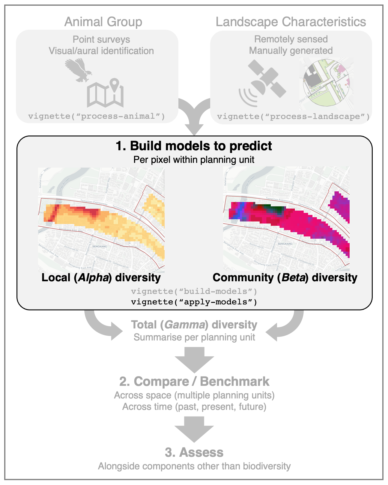
apply-models.RmdThis article outlines the steps to predict the diversity of a
particular animal group across a target landscape. The pixel-based
predictions can then be visualised spatially as a raster image. Based on
community ecology theory, we ‘decompose’ animal diversity into two
components: (1) local (Alpha) diversity and (2) community
(Beta) diversity. The example models built in
vignette("build-models") will be used in this
demonstration.
1. Local (Alpha) diversity
First, load the required packages:
library("biodivercity")
library("dplyr") # to process/wrangle data
library("tmap") # for visualisation
In this article, we will make spatial predictions across the Punggol
(PG) area in Singapore, taken from the example dataset
sampling_areas.
# load polygon of punggol boundaries
data(sampling_areas)
punggol <- sampling_areas %>%
   filter(area == "PG")

# get landscape data ready
filepath <- system.file("extdata", "osm_data.Rdata", package = "biodivercity")
load(filepath)

ndvi_mosaic <-
  system.file("extdata", "ndvi_mosaic.tif", package="biodivercity") %>%
  terra::rast()
veg_classified <- classify_image_binary(ndvi_mosaic, threshold = "otsu")

# visualise
tmap_mode("view")
tm_basemap(c("CartoDB.Positron")) +
  tm_shape(punggol) + tm_borders() +
  tm_shape(buildings_osm) + tm_polygons(col = "levels") +
  tm_shape(roads_osm) + tm_lines(col = "lanes", palette = "YlOrRd")+
  tm_shape(veg_classified) +
    tm_raster(style = "cat",
            palette = c("grey", "darkgreen"))
Next, load the model object and extract the landscape predictors within the best models. In this example, the largest radius for variables within the models is 400 metres.
filepath <- system.file("extdata", "apply-models_alpha-diversity.Rdata", package="biodivercity")
load(filepath)

# landscape predictors
predictors <- colnames(coef(bestmodels_info)[,-1])
predictors
## [1] "r200m_lsm_veg_gyrate_mn" "r200m_osm_buildingVol_m3"
## [3] "r200m_osm_laneDensity" "r200m_lsm_veg_area_mn"
## [5] "r200m_lsm_veg_ed" "r400m_lsm_veg_ed"
## [7] "r400m_osm_buildingFA_ratio" "r200m_lsm_veg_lpi"
## [9] "r200m_osm_buildingFA_ratio"
# get the max radius among all predictor variables
max_radius <- predictors %>%
  stringr::str_extract("(?<=^r)\\d+") %>%  # extract buffer radii
  as.numeric() %>%
  max(na.rm = TRUE)
max_radius
## [1] 400To make spatial predictions, the target area is broken up into many
smaller points (pixels), where landscape data will be summarised and
predictions will be made. First, use the function
generate_grid() to generate a grid over the target
area.
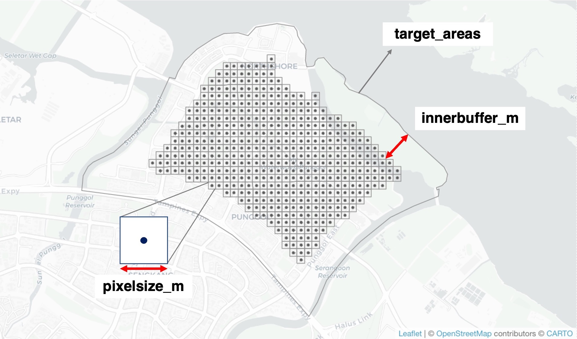
Figure: Visualisation of the function generate_grid().
The pixel resolution of the grid can be customised with the argument
pixelsize_m, which we specify as 100 metres in this
example. An optional argument innerbuffer_m limits the
spatial predictions to a smaller area within the target landscape. This
is useful, for example, when the model requires broad-scale landscape
data to make predictions, but available landscape data do not extend
beyond the target area. Hence, to avoid inaccurate predictions that
result from areas without landscape data, the distance value for this
argument should correspond to the largest buffer radius present in the
model variables.
grid_points <- generate_grid(target_areas = punggol,
                             pixelsize_m = 100,
                             innerbuffer_m = max_radius) %>%
  rownames_to_column("point_id") # add unique identifier

grid_points # geometry column has been added
## Simple feature collection with 461 features and 2 fields
## Geometry type: POINT
## Dimension: XY
## Bounding box: xmin: 377114.5 ymin: 153973.6 xmax: 380414.5 ymax: 156673.6
## Projected CRS: WGS 84 / UTM zone 48N
## First 10 features:
## point_id area geometry
## 1 1 PG POINT (379114.5 153973.6)
## 2 2 PG POINT (379014.5 154073.6)
## 3 3 PG POINT (379114.5 154073.6)
## 4 4 PG POINT (379214.5 154073.6)
## 5 5 PG POINT (378914.5 154173.6)
## 6 6 PG POINT (379014.5 154173.6)
## 7 7 PG POINT (379114.5 154173.6)
## 8 8 PG POINT (379214.5 154173.6)
## 9 9 PG POINT (379314.5 154173.6)
## 10 10 PG POINT (378914.5 154273.6)At each grid point, summarise the predictors for land cover and
OpenStreetMap data using the functions calc_specific_lsm()
and calc_specific_osm(), respectively. Each predictor will
be summarised within the relevant distance buffer (radius) from the grid
point, denoted by the prefix r<value>m. If manually
generated landscape data were used and are present within the best
models, the function calc_manual() can be used to summarise
each landscape component; see vignette("process-landscape")
for the full list of landscape vectors that may be summarised.
# vegetation cover
predictors_veg <- stringr::str_subset(predictors, "lsm_veg_.*$")
results_veg <-
  calc_specific_lsm(raster = veg_classified,
                    predictors_lsm = predictors_veg,
                    class_names = c("veg"),
                    class_values = c(1),
                    points = grid_points)

# osm buildings
predictors_buildings <- stringr::str_subset(predictors, "osm_building.*$")
results_buildings <-
      calc_specific_osm(vector = buildings_osm,
                        predictors_osm = predictors_buildings,
                        building_levels = "levels",
                        building_height = "height",
                        points = grid_points)

# osm roads
predictors_roads <- stringr::str_subset(predictors, "osm_lane.*$")
results_roads <-
      calc_specific_osm(vector = roads_osm,
                        predictors_osm = predictors_roads,
                        road_lanes = "lanes",
                        points = grid_points)

# combine results and overwrite 'grid_points' variable
grid_points <- results_veg %>%
  full_join(results_buildings %>% st_set_geometry(NULL)) %>%
  full_join(results_roads %>% st_set_geometry(NULL))
grid_points
## Simple feature collection with 461 features and 11 fields
## Geometry type: POINT
## Dimension: XY
## Bounding box: xmin: 377114.5 ymin: 153973.6 xmax: 380414.5 ymax: 156673.6
## Projected CRS: WGS 84 / UTM zone 48N
## First 10 features:
## point_id area r200m_lsm_veg_area_mn r200m_lsm_veg_ed r400m_lsm_veg_ed
## 1 1 PG 0.1783333 304.3825 287.8758
## 2 2 PG 0.3790909 273.3068 320.5256
## 3 3 PG 0.2118750 292.4303 310.9695
## 4 4 PG 0.1394737 278.8845 295.8391
## 5 5 PG 0.2653846 307.5697 329.2853
## 6 6 PG 0.3911111 267.7291 331.4752
## 7 7 PG 0.4800000 280.4781 321.9192
## 8 8 PG 0.2733333 248.6056 308.9787
## 9 9 PG 0.1822222 306.7729 293.2510
## 10 10 PG 0.2193333 332.2709 335.4569
## r200m_lsm_veg_gyrate_mn r200m_lsm_veg_lpi r200m_osm_buildingVol_m3
## 1 18.12023 10.677291 0
## 2 25.96049 18.964143 0
## 3 18.32125 14.501992 0
## 4 12.40779 13.386454 0
## 5 18.90708 12.191235 0
## 6 23.45344 18.884462 0
## 7 25.94185 24.302789 0
## 8 16.08908 18.406375 0
## 9 15.67557 13.227092 0
## 10 19.89673 9.800797 0
## r400m_osm_buildingFA_ratio r200m_osm_buildingFA_ratio r200m_osm_laneDensity
## 1 1.682808 1.623362 0.04645401
## 2 2.233960 2.700053 0.02081570
## 3 1.946201 2.615702 0.02345348
## 4 1.714228 2.362860 0.03613221
## 5 2.438732 3.239166 0.03077676
## 6 2.411402 3.061500 0.02277422
## 7 2.194357 3.041585 0.01304752
## 8 1.861286 3.370845 0.01692167
## 9 1.695405 2.670577 0.02997526
## 10 2.603705 3.244310 0.03184894
## geometry
## 1 POINT (379114.5 153973.6)
## 2 POINT (379014.5 154073.6)
## 3 POINT (379114.5 154073.6)
## 4 POINT (379214.5 154073.6)
## 5 POINT (378914.5 154173.6)
## 6 POINT (379014.5 154173.6)
## 7 POINT (379114.5 154173.6)
## 8 POINT (379214.5 154173.6)
## 9 POINT (379314.5 154173.6)
## 10 POINT (378914.5 154273.6)Finally, use the function predict_heatmap() to predict
the number of bird species (species richness) across the grid of spatial
points, based on the predictor variables summarised in
grid_points. The model object(s) in bestmodels
(lme4::glmer() objects) and recipe_birds (data
pre-processing workflow recipes::recipe() object) will be
used to make the predictions at each point. Ensure that the argument
pixelsize_m is similar to the value used in
generate_grid().
bird_heatmap <- predict_heatmap(models = bestmodels,
                                recipe_data = recipe_birds,
                                points_topredict = grid_points,
                                pixelsize_m = 100)
The continuous raster may be visualised as a heat map:
tmap_options(max.raster = c(view = 1e8)) # increase max resolution to be visualised

tm_basemap(c("CartoDB.Positron", "OpenStreetMap")) +
  tm_shape(bird_heatmap, raster.downsample = FALSE) +
  tm_raster(title = "Number of bird species",
            style = "pretty",
            n = 8,
            palette = "YlOrRd",
            alpha = 0.6)