Model Use Cases

1. Citywide monitoring

Models that are built using remotely sensed data can be used to predict the diversity of an animal group across different time periods and across large areas. For example, if remotely sensed data across an entire city is available, spatial predictions can be generated citywide (see vignette("apply-models")). Depending on the level of detail required, the pixel resolution can be adjusted accordingly.

Load the example data for predictions of bird local (Alpha) diversity across the city of Singapore during the year 2020:

bird_heatmap <- 
  system.file("extdata", "alpha-diversity_birds_delta-aic-2_subzones_500m.tif", package="biodivercity") %>% 
  terra::rast()


# load zones used in city planning
sg_subzones <- 
  system.file("extdata", "sg_subzones.geojson", package="biodivercity") %>% 
  read_sf() %>% 
  relocate("subzone_n")


# plot map
tmap_mode("view")
tm_basemap(c("CartoDB.Positron")) +
  tm_shape(sg_subzones) +
    tm_polygons(group = "Singapore Subzones",
                alpha = 0) +
  tm_shape(bird_heatmap, raster.downsample = FALSE) +
    tm_raster(group = "Local diversity: Birds",
              title = "Number of bird species",
              style = "fisher",
              n = 8,
              palette = "YlOrRd",
              alpha = 0.6)

Map: Spatial predictions of local diversity of birds across subzones in Singapore. The pixel resolution used for predictions in this example is 500 m x 500 m.

Pixel values within the zones used in city planning can be summarised, to allow comparisons to be made between these planning units. The resulting distribution of the summarised values can subsequently be used to compare the ‘performance’ of each planning unit relative to others in the city, or to a set a benchmark/target for the desired level of ‘performance’. For example, subzones in Singapore could be benchmarked against the mean of the distribution, as shown below:

to_plot <- sg_subzones %>% 
  dplyr::mutate(bird_alpha_mean = # calc mean alpha diversity per subzone
                  terra::extract(bird_heatmap,terra:::vect(sg_subzones), 
                                 fun = "mean", na.rm = TRUE) %>% 
           dplyr::mutate(predicted = ifelse(is.nan(predicted), NA, predicted)) %>% 
           dplyr::pull(predicted))


# set benchmark & range of values for scoring 
benchmark <- to_plot %>% 
  dplyr::summarise(mean = mean(bird_alpha_mean, na.rm = TRUE),
                   sd = sd(bird_alpha_mean, na.rm = TRUE)) %>% 
  sf::st_set_geometry(NULL)
distribute_sd <- c(-1.5,-0.5,0.5,1.5) # score based on st dev from the mean

# for visualisation of the scoring regions
data_regions <- 
  data.frame(start = c(benchmark$mean + head(distribute_sd, 1)*benchmark$sd-50, # start well below the minimum value
                       benchmark$mean + distribute_sd*benchmark$sd),
             end = c(benchmark$mean + distribute_sd*benchmark$sd,
                     benchmark$mean + tail(distribute_sd, 1)*benchmark$sd+50), # end will above the max value
             Score = factor(0:4)) # arbitrary score of 0-4

# plot
to_plot %>%
  drop_na(bird_alpha_mean) %>% 
  ggplot() +
    geom_rect(data = data_regions,
            aes(xmin = start,
                xmax = end,
                ymin = - Inf,
                ymax = Inf,
                fill = Score),
            alpha = 0.5) +
    geom_histogram(aes(x = bird_alpha_mean), bins = 30, binwidth = 1.0) + 
    geom_label(data = data_regions[1>4,],
               aes(label = paste(distribute_sd, "SD"), 
                   x = head(data_regions$end, 4),
                   y = 1.0),
               size = 3.0,
               label.padding = unit(0.15, "lines")) +
    coord_cartesian(xlim=c(min(to_plot$bird_alpha_mean, na.rm = TRUE) - 1, 
                           max(to_plot$bird_alpha_mean, na.rm = TRUE) + 1)) +
  
    scale_x_continuous(breaks = scales::breaks_pretty(n = 6)) +
    scale_y_continuous(breaks = scales::breaks_pretty(n = 3), 
                       limits = c(NA, 45),
                       expand = c(0, 0)) +
    scale_fill_brewer(type = "div", palette = "Greens") +
    xlab("Average no. of bird species per pixel") +
    ylab("Frequency (No. of subzones)") +
    theme_bw() +
    theme(panel.grid.minor.x = element_blank(),
          panel.grid.major.x = element_blank(),
          panel.grid.minor.y = element_blank(),
          legend.text.align = 1)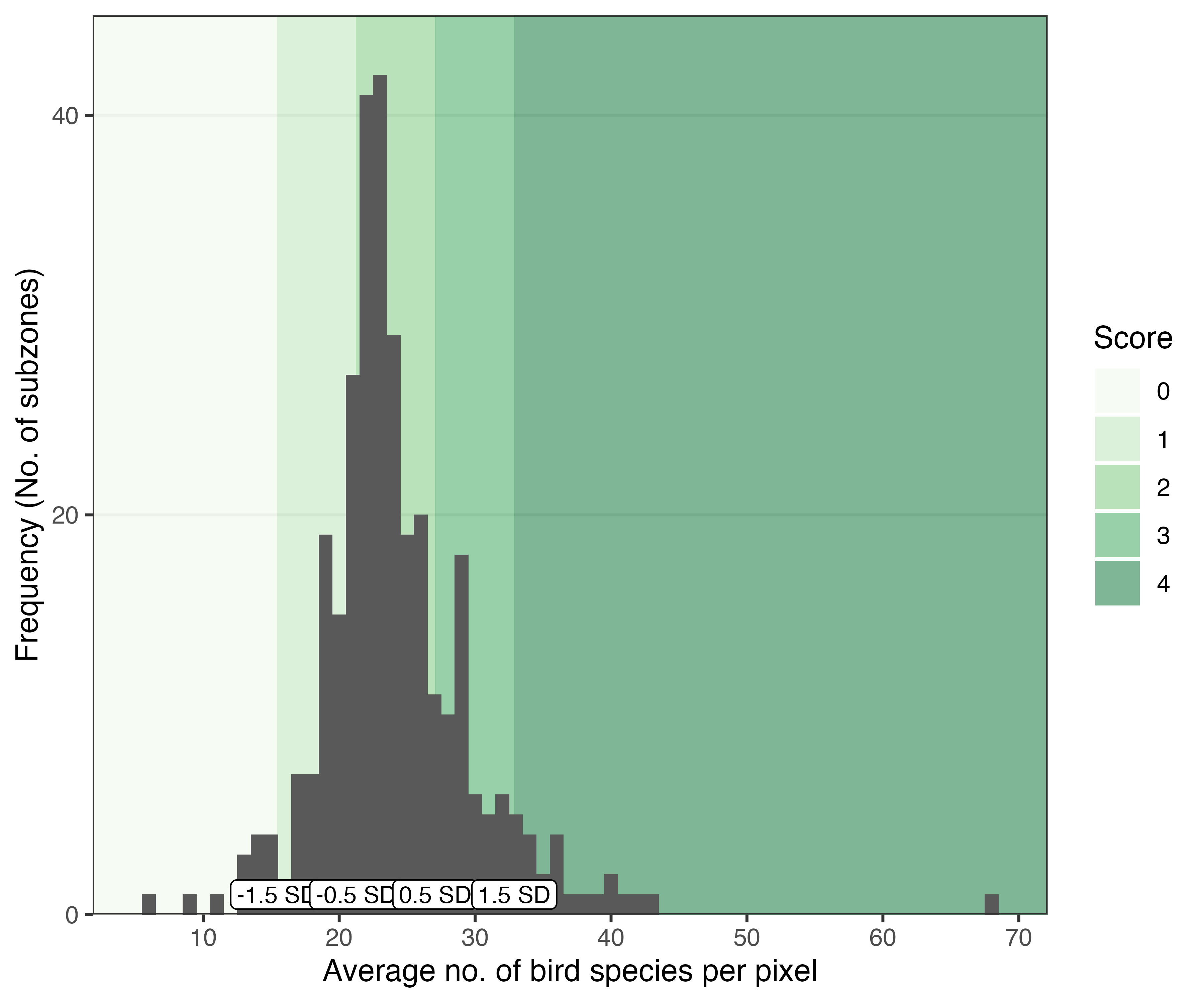

Histogram showing the distribution of values for the mean number of bird species per pixel within each of the 332 subzones in Singapore. Subzones were assigned an arbitrary score of 0-4 based on standard deviations from the mean (i.e., performance of the ‘average’ subzone).

If spatial predictions were made for multiple snapshots in time, benchmarking could be based on whether the average pixel value for a particular planning unit increases or decreases between two time periods. For example, if ‘no net loss’ in biodiversity is set as a target, a negative score could be assigned if the average pixel value is reduced, while a positive score could be assigned if the average pixel value increases.

Finally, it is worth noting that full customisation of both the pixel size and boundaries within which to summarise the pixel values can be done. This provides flexibility according to the level of analysis (e.g., geographical scale) required by the user. By summarising pixel values within zones used in city planning, animal diversity may be assessed alongside other indices also summarised at the level of these planning units, thus providing a more comprehensive view of components related to biodiversity and beyond.

2. Biodiversity in the future

Other than monitoring changes in biodiversity, there is also a need to assess future urban developments, for instance, to see if proposed designs can effectively mitigate the loss of biodiversity. But since such landscapes do not exist, snapshots of remotely sensed data can not be used. It is therefore important to carefully consider data compatibility between these different use cases when building and using the predictive models.

Urban design and planning involves the consideration of multiple design scenarios. Manually generated landscape elements (e.g., vector data for vegetation) may be produced from prospective designs, but the format and types of such data must be compatible with those used in the predictive models. For instance, when selecting landscape predictors to build the models, land cover classification as discrete rasters would be more compatible with manually generated data, compared to continuous rasters that cannot be feasibly calculated (e.g., spectral indices such as NDVI). Vegetation generated in design scenarios can be rasterized into discrete land cover-types (see Figure below), and used to replace the remotely sensed data within regions of interest (see Interactive Map below). Such amendments to landscape data can be made across a site slated for urban development, and then used to make spatial predictions for that particular design scenario.

Example showing how manually generated vector data of vegetation can be converted into a classified raster of vegetation types used in the predictive models.

To demonstrate this, we can import remotely-sensed data within the Punggol (PG) area in Singapore. The following code are very similar to the examples shown in vignette("apply-models").

# load polygon of punggol boundaries
data(sampling_areas)
punggol <- sampling_areas %>%
   filter(area == "PG")

# get landscape data ready
filepath <- system.file("extdata", "osm_data.Rdata", package = "biodivercity")
load(filepath)

ndvi_mosaic <- system.file("extdata", "ndvi_mosaic.tif", package="biodivercity") %>% 
  terra::rast()
veg_remote <- classify_image_binary(ndvi_mosaic, threshold = "otsu")

Next, import landscape vectors (points, polygons, lines) mapped manually within a site in PG (Chong et al., 2014, 2019). These represent manually generated data from a design scenario. Further details and a visualisation of these vector data are available in vignette("process-landscape").

filepath <- system.file("extdata", "landscape-vectors_mapped.Rdata", package = "biodivercity") # load example data
load(filepath)

With the remotely sensed data across the broader PG area and manually generated data within the site of interest, we can replace (amend) the original data within the site with the (rasterised) vector data. In this simple demonstration, we project the canopy area of each tree (point) based on a 5m radius, and combine all manually mapped vegetation into a single class (category).

# combine all veg vectors
veg <- trees %>% 
  st_buffer(dist = 5) %>%  # 5m radius for tree canopies
  bind_rows(natveg) %>% 
  bind_rows(shrubs) %>% 
  bind_rows(turf)

# rasterise veg vectors
veg_rasterised <- 
  terra::rasterize(terra::vect(veg),
                   veg_remote, # use remotely sensed vegetation as reference raster
                   background = 0) 

# mask away rasterised veg not within site boundaries
veg_rasterised <- 
       terra::mask(veg_rasterised, 
                   vect(bound))

# mask away the site from remotely sensed veg
veg_amended <- terra::mask(veg_remote, vect(bound), inverse = TRUE)
  
# fill in amended veg raster with rasterised veg
veg_amended <- terra::mosaic(veg_amended, veg_rasterised)

Similarly, building and roads within the site boundaries are replaced (amended).

# buildings
buildings_amended <- buildings_osm %>% 
  sf::st_difference(sf::st_union(bound)) %>% # remove osm buildings within site boundaries
  dplyr::mutate(source = "osm") %>% # add column indicating data source
  bind_rows(buildings %>% # append manually generate buildings
              mutate(source = "generated"))

# roads
roads_amended <- roads_osm %>% 
  sf::st_difference(sf::st_union(bound)) %>% # remove osm roads within site boundaries
  mutate(lanes = as.numeric(lanes)) %>% 
  dplyr::mutate(source = "osm") %>% # add column indicating data source
  bind_rows(roads %>% # append manually generate buildings
              mutate(source = "generated"))

Here’s map showing both the original and amended rasters for classified vegetation:

Map: Example showing how a classified raster of remotely sensed vegetation can be amended with the manually generated (rasterised) vector data at a site (red boundaries) within Punggol, Singapore. Toggle the map layers to view the amended raster layer.

Following similar code in vignette("apply-models"), these amended data for vegetation, buildings and roads can then be used to make spatial predictions of animal diversity across the site of interest. In the example below, we show how local (Alpha) bird diversity can be predicted for the original and amended scenario. The process within this vignette can be repeated accordingly if there are multiple design scenarios.

Process the model data and generate a regular grid across the site of interest:

filepath <- system.file("extdata", "apply-models_alpha-diversity.Rdata", package="biodivercity")
load(filepath)

# landscape predictors
predictors <- colnames(coef(bestmodels_info)[,-1])

# generate regular grid within site boundaries
grid_points <- generate_grid(target_areas = bound, 
                             pixelsize_m = 50,
                             innerbuffer_m = 0) %>%
  rownames_to_column("point_id") # add unique identifier

Make predictions for the original dataset:

# vegetation cover
predictors_veg <- stringr::str_subset(predictors, "lsm_veg_.*$")
results_veg <- 
  calc_specific_lsm(raster = veg_remote,
                    predictors_lsm = predictors_veg,
                    class_names = c("veg"),
                    class_values = c(1),
                    points = grid_points,
                    na_threshold = 0) # reduce no. of NA pixels, since original & amended scenarios have no data outside the site boundaries 

# osm buildings
predictors_buildings <- stringr::str_subset(predictors, "osm_building.*$")
results_buildings <-
      calc_specific_osm(vector = buildings_osm,
                        predictors_osm = predictors_buildings,
                        building_levels = "levels",
                        building_height = "height",
                        points = grid_points)

# osm roads
predictors_roads <- stringr::str_subset(predictors, "osm_lane.*$")
results_roads <-
      calc_specific_osm(vector = roads_osm,
                        predictors_osm = predictors_roads,
                        road_lanes = "lanes",
                        points = grid_points)

# combine results and overwrite 'grid_points' variable 
grid_points_original <- results_veg %>% 
  full_join(results_buildings %>% st_set_geometry(NULL)) %>% 
  full_join(results_roads %>% st_set_geometry(NULL))

# make predictions
bird_heatmap <- 
  predict_heatmap(models = bestmodels, 
                  recipe_data = recipe_birds,
                  points_topredict = grid_points_original, 
                  pixelsize_m = 50)

Make predictions for the amended dataset:

# vegetation cover
predictors_veg <- stringr::str_subset(predictors, "lsm_veg_.*$")
results_veg_amended <- 
  calc_specific_lsm(raster = veg_amended,
                    predictors_lsm = predictors_veg,
                    class_names = c("veg"),
                    class_values = c(1),
                    points = grid_points,
                    na_threshold = 0) # reduce no. of NA pixels, since original & amended scenarios have no data outside the site boundaries 

# osm buildings
predictors_buildings <- stringr::str_subset(predictors, "osm_building.*$")
results_buildings_amended <-
      calc_specific_osm(vector = buildings_amended,
                        predictors_osm = predictors_buildings,
                        building_levels = "levels",
                        building_height = "height",
                        points = grid_points)

# osm roads
predictors_roads <- stringr::str_subset(predictors, "osm_lane.*$")
results_roads_amended <-
      calc_specific_osm(vector = roads_amended,
                        predictors_osm = predictors_roads,
                        road_lanes = "lanes",
                        points = grid_points)

# combine results and overwrite 'grid_points' variable 
grid_points_amended <- results_veg_amended %>% 
  full_join(results_buildings_amended %>% st_set_geometry(NULL)) %>% 
  full_join(results_roads_amended %>% st_set_geometry(NULL))

# make predictions
bird_heatmap_amended <- 
  predict_heatmap(models = bestmodels, 
                  recipe_data = recipe_birds,
                  points_topredict = grid_points_amended, 
                  pixelsize_m = 50)

The predictions for both scenarios are shown below as heat maps. Toggle the map layers to view predictions based on the amended landscape data.

Map: Spatial predictions of local (Alpha) diversity of birds at a site (red boundaries) within Punggol, Singapore. The pixel resolution used for predictions in this example is 10 m x 10 m. The color palettes were binned based on the Jenks natural breaks classification.

Similar to the previous section, the pixel values across a site can be summarised (e.g. calculate the mean pixel value). For a given site, summarised values between different scenarios can be compared based on their local (Alpha) and community (Beta) diversity, as well as other indices that may not be related to biodiversity.

To conclude, while such data conversions may allow similar predictors (and hence models) to be used for different use cases, it should be noted that potential mismatches between different data sources may result in inaccurate predictions. Reducing the mismatch between remotely sensed and manually generated data is an important gap that should be addressed. For instance, the level of detail in design scenarios may not include the exact locations of planted trees, and their estimated canopy projection areas may vary greatly from reality after planting. Furthermore, the remotely sensed data represents a top-down view of the landscape, and the effect of multi-tiered planting is not accounted for within the landscape predictors. Communication with practitioners is needed to ensure that model workflows align with the data formats and outputs used in design practice, and that suitable methods are used to ensure that artificially generated datasets are both compatible and accurate to reality after implementation.

References

Chong KY, Teo S, Kurukulasuriya B, Chung YF, Giam X & Tan HTW (2019) The effects of landscape scale on greenery and traffic relationships with urban birds and butterflies. Urban Ecosystems, 22(5): 917–926.

Chong KY, Teo S, Kurukulasuriya B, Chung YF, Rajathurai S & Tan HTW (2014) Not all green is as good: Different effects of the natural and cultivated components of urban vegetation on bird and butterfly diversity. Biological Conservation, 171: 299–309.

Government of Singapore (2020). Master Plan 2019 Subzone Boundary (No Sea). data.gov.sg Released under the terms of the Singapore Open Data Licence version 1.0.

Quantitative comparisons of animal diversity across space and time

2022-12-08

1. Citywide monitoring

2. Biodiversity in the future

References