Build Models

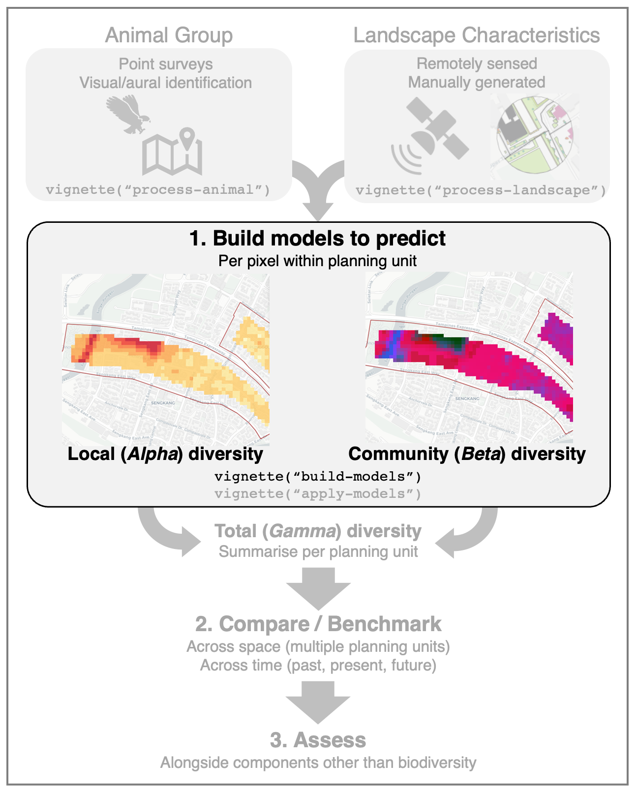
This article outlines a workflow to build predictive models of diversity for a chosen animal group. Fauna and landscape data should have already been prepared based on vignette("process-animal") and vignette("process-landscape"), respectively. Based on community ecology theory, we ‘decompose’ animal diversity into two components: (1) local (Alpha) diversity and (2) community (Beta) diversity. A predictive model will be built for each component.

Figure: Broad overview of the data workflow for a chosen animal group

First, load the necessary packages used throughout this article:

library("biodivercity")
library("tidyverse") # to process/wrangle data
library("sf") # to process landscape data

1. Local (Alpha) diversity

For a chosen animal group, local (Alpha) diversity is represented by the number of species recorded at sampling point locations (i.e., species density). The response variable is the number (count) of species. Generalised linear mixed-effects models (GLMMs) can be used to model count data, and linear models are generally simpler and provide better interpretability. Do note that other types of models/algorithms can also be used to model count data. Also, the full list of potential predictor variables may first be narrowed down; for example, random forest models may be used to select variables based on their relative importance in improving model performance (Arthur et al., 2010; Li et al., 2017).

Load the necessary packages to model local (Alpha) diversity:

library("lme4") # mixed-effects modelling
library("MuMIn") # model selection & averaging

Load the example datasets for birds (animal group ‘Aves’) recorded at sampling points across Singapore. birds is a dataframe containing the number of species aggregated across multiple surveys (i.e., species richness; column ‘sprich’), and landscape is a dataframe containing landscape predictors summarised within specified buffer radii. These example datasets can be obtained by following the steps in vignette(process-animal) and vignette(process-landscape), respectively. See data(animal_surveys) and data(points_landscape) for further details about the underlying animal and landscape data.

filepath <- system.file("extdata", "build-models_alpha-diversity.Rdata", package="biodivercity")
load(filepath)

Pivot the landscape_data to wide format, with the prefix r<radius>m_ (representing the radius size) appended to the column names of predictors:

landscape <- landscape %>% 
  pivot_longer(cols = c(starts_with("osm_"), starts_with("lsm_")),
               names_to = 'metric') %>% 
  pivot_wider(id_cols = c("town", "point_id"),
              names_from = c("radius_m", "metric"), 
              values_from = "value",
              names_glue = "r{radius_m}m_{metric}")

# combine bird and landscape data, then then scale/center variables
birds <- birds %>% 
  inner_join(landscape, by = c("town", "point_id")) 
birds_scaled <- birds %>% 
  mutate(across(.cols = where(is.numeric) & !sprich, scale))

head(birds_scaled) # view combined data

## # A tibble: 6 × 20
##   town  priority point…¹ sprich r200m_…² r200m…³ r200m…⁴ r200m…⁵ r200m…⁶ r200m…⁷
##   <chr> <chr>    <chr>    <int>    <dbl>   <dbl>   <dbl>   <dbl>   <dbl>   <dbl>
## 1 PG    Aves     PGT15       14  0.00303  0.575    0.694  -0.497  -0.559   0.456
## 2 PG    Aves     PGT14       21  0.852    0.344    1.72   -0.485  -0.496   0.621
## 3 PG    Aves     PGT6        21  1.66     0.997    2.71   -0.511  -0.544   1.01 
## 4 QT    Aves     QTNa14…     34 -1.17    -0.0279  -0.740   3.54    3.40   -0.859
## 5 QT    Aves     QTNb1a…     40 -1.35    -0.948   -0.799   1.60    1.31   -1.97 
## 6 PG    Aves     PGT7        18  1.33     0.801    2.52   -0.472  -0.490   0.440
## # … with 10 more variables: r200m_lsm_veg_lpi <dbl[,1]>,
## #   r200m_lsm_veg_pland <dbl[,1]>, r400m_osm_buildingVol_m3 <dbl[,1]>,
## #   r400m_osm_laneDensity <dbl[,1]>, r400m_osm_buildingFA_ratio <dbl[,1]>,
## #   r400m_lsm_veg_area_mn <dbl[,1]>, r400m_lsm_veg_gyrate_mn <dbl[,1]>,
## #   r400m_lsm_veg_ed <dbl[,1]>, r400m_lsm_veg_lpi <dbl[,1]>,
## #   r400m_lsm_veg_pland <dbl[,1]>, and abbreviated variable names ¹point_id,
## #   ²r200m_osm_buildingVol_m3[,1], ³r200m_osm_laneDensity[,1], …

To fit the model as a GLMM, the function MuMIn::dredge() will be used. The function includes customisation options; for instance, the subset argument allows the user to exclude certain combinations of variables within the fitted model (i.e., apply constraints to possible models that may be built). In the following example, we do not allow the same landscape predictor summarised within multiple buffer radii to be present in the same model.

predictors <- grep("^r[0-9]+m_",  colnames(birds_scaled), value = TRUE) # get predictor names

# get rows with same predictors but different radii
var_comb <- combn(predictors, 2) %>% # unique combinations
  t() %>% 
  as.data.frame() %>%  # separate radii & predictors
  separate(V1, c("V1_radius", "V1_predictor"),
           sep = "(?<=[0-9])m_(?=[A-Za-z]*)", remove = FALSE) %>% 
  separate(V2, c("V2_radius", "V2_predictor"),
           sep = "(?<=[0-9])m_(?=[A-Za-z]*)", remove = FALSE) %>%
  rowwise() %>% 
  mutate(similar = grepl(V1_predictor, V2_predictor)) %>% 
  filter(isTRUE(similar))

# create object to be supplied to function argument
subset_vect <- paste(var_comb$V1, "&", var_comb$V2)
subset_exp <- parse(text = paste0("!(", paste(subset_vect, collapse = ") & !("), ")")) # function argument requires an expression

Next, we fit both a global (maximal) model and null model, in order to calculate the difference in Akaike Information Criterion (AIC) value within the function MuMIn::dredge(). In the example data, the ‘town’ is specified as the random effect. The argument ‘family’ is specified as "poisson", since the response variable is count data. See the function lme4::glmer() for more details and information on its arguments.

model_global <- 
  glmer(paste("sprich", "~", paste(predictors, collapse = " + "), 
              "+ (1|town) "),
        family = "poisson",
        na.action = "na.fail",
        control = lme4::glmerControl(optimizer = "bobyqa"),
        data = birds_scaled)

model_null <- 
  glmer(sprich ~ 1 + (1|town), family = "poisson", data = birds_scaled)

Automated model selection is performed using the function MuMIn::dredge(). Models are ranked based on their AICc value (AIC adjusted for small sample sizes). Model constraints are specified in the argument subset. To avoid a long runtime in this demonstration, we also limit the number of predictor variables in each model to four (argument m.lim).

model_glm <- dredge(model_global,
                    subset= subset_exp,
                    m.lim=c(NA,4), # max of 4 variables
                    rank="AICc")

The resulting object contains a model selection table, with each row representing a model that was fit. It is arranged in ascending order, based on AIC value (lower AIC value represents a ‘better’ model). A summary of the top models with values of ΔAIC < 2 can be viewed:

bestmodels_info <- subset(model_glm, 
                         delta < 2, 
                         recalc.weights=FALSE)

knitr::kable(bestmodels_info, caption = "**Summary of best models ranked based on automated model selection from `MuMIn::dredge()` (ΔAIC < 2).**") %>%
  kableExtra::kable_styling("striped") %>% kableExtra::scroll_box(width = "100%", height = "300px")

**Summary of best models ranked based on automated model selection from `MuMIn::dredge()` (ΔAIC < 2).**
	(Intercept)	r200m_lsm_veg_area_mn	r200m_lsm_veg_ed	r200m_lsm_veg_gyrate_mn	r200m_lsm_veg_lpi	r200m_lsm_veg_pland	r200m_osm_buildingFA_ratio	r200m_osm_buildingVol_m3	r200m_osm_laneDensity	r400m_lsm_veg_area_mn	r400m_lsm_veg_ed	r400m_lsm_veg_gyrate_mn	r400m_lsm_veg_lpi	r400m_lsm_veg_pland	r400m_osm_buildingFA_ratio	r400m_osm_buildingVol_m3	r400m_osm_laneDensity	df	logLik	AICc	delta	weight
197	3.196216	NA	NA	0.0551637	NA	NA	NA	-0.1359401	-0.0850794	NA	NA	NA	NA	NA	NA	NA	NA	5	-365.8589	742.2395	0.0000000	0.05939683
194	3.196120	0.0514166	NA	NA	NA	NA	NA	-0.1412017	-0.0832377	NA	NA	NA	NA	NA	NA	NA	NA	5	-366.1590	742.8397	0.6002541	0.04399666
199	3.195786	NA	-0.0256461	0.0461363	NA	NA	NA	-0.1280837	-0.0802518	NA	NA	NA	NA	NA	NA	NA	NA	6	-365.3751	743.4871	1.2475980	0.03183104
709	3.196645	NA	NA	0.0488160	NA	NA	NA	-0.1267322	-0.0812710	NA	-0.0231842	NA	NA	NA	NA	NA	NA	6	-365.4697	743.6763	1.4368451	0.02895718
8389	3.195210	NA	NA	0.0542352	NA	NA	NA	-0.1271918	-0.0833486	NA	NA	NA	NA	NA	-0.0209911	NA	NA	6	-365.5583	743.8534	1.6139420	0.02650332
205	3.195503	NA	NA	0.0447909	0.0269169	NA	NA	-0.1262190	-0.0771083	NA	NA	NA	NA	NA	NA	NA	NA	6	-365.5612	743.8592	1.6196856	0.02642731
229	3.195477	NA	NA	0.0553025	NA	NA	-0.0183244	-0.1260268	-0.0838809	NA	NA	NA	NA	NA	NA	NA	NA	6	-365.6520	744.0408	1.8013640	0.02413249
196	3.195746	0.0419566	-0.0251969	NA	NA	NA	NA	-0.1331441	-0.0792678	NA	NA	NA	NA	NA	NA	NA	NA	6	-365.7112	744.1592	1.9197703	0.02274524
706	3.196583	0.0449303	NA	NA	NA	NA	NA	-0.1311233	-0.0796107	NA	-0.0241621	NA	NA	NA	NA	NA	NA	6	-365.7387	744.2143	1.9747749	0.02212821

We can also visualise the importance (based on sum-of-weights) and effect direction (based on coefficient value) for each variable within the top models:

# average the effect of each predictor
effects <- data.frame(coef(bestmodels_info)[,-1]) %>% 
  summarise(across(everything(), ~ mean(.x, na.rm = TRUE))) %>% 
  pivot_longer(everything(), names_to = "var") %>% 
  mutate(effect = ifelse(value > 0, "Positive", "Negative"))

# get importance of each predictor
importances <- data.frame(MuMIn::sw(bestmodels_info)) %>% 
  rename(imp = MuMIn..sw.bestmodels_info.) %>% 
  rownames_to_column("var") %>% 
  left_join(effects, by = "var") %>% # join with effects
  mutate(effect = ifelse(is.na(effect), "Mixed (factor)", effect)) %>%
  mutate(effect = factor(effect, levels = c("Positive", "Negative", "Mixed (factor)")))

# plot
ggplot(data=importances, aes(x = imp, y = reorder(var, imp), 
                     fill = effect)) + 
  geom_bar(stat = "identity") +
  labs(x = "Sum of weights", y = "Variables") +
  scale_fill_manual(values = c("#4daf4a", "#e41a1c", "#377eb8"),
                    name = "Effect")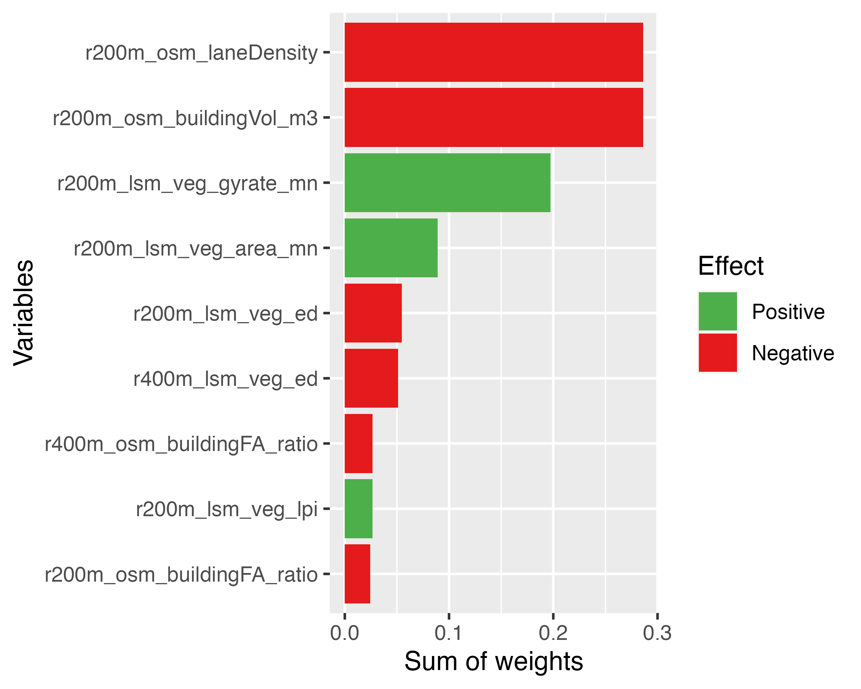

Finally, we can extract the models and recipes::recipe() objects for future use:

# get list of best models
bestmodels <- MuMIn::get.models(bestmodels_info, subset = TRUE)

# create recipes object only with predictors within best models
predictors_best <- colnames(coef(bestmodels_info)[,-1])

birds <- birds %>% # original unscaled dataset
  dplyr::select(sprich, town, all_of(predictors_best)) # remove unnecessary columns

recipe_birds <- recipes::recipe(birds) %>% 
  recipes::update_role(sprich, new_role = "outcome") %>%
  recipes::update_role(town, new_role = "id") %>%
  recipes::update_role_requirements("id", bake = FALSE) %>%
  recipes::step_normalize(all_of(predictors_best)) %>% 
  recipes::prep()

2. Community (Beta) diversity

To be released.

References

Arthur AD, Li J, Henry S & Cunningham SA (2010) Influence of woody vegetation on pollinator densities in oilseed Brassica fields in an Australian temperate landscape. Basic and Applied Ecology, 11(5): 406–414.

Li J, Alvarez B, Siwabessy J, Tran M, Huang Z, Przeslawski R, Radke L, Howard F & Nichol S (2017) Application of random forest and generalised linear model and their hybrid methods with geostatistical techniques to count data: Predicting sponge species richness. Environmental Modelling and Software, 97: 112–129.

Train models that predict animal diversity from landscape data

2022-12-08

1. Local (Alpha) diversity

2. Community (Beta) diversity

References