Animals: Simulate Missing Surveys

Visualise the reduction in number of animal species if surveys are missed

2022-12-08

Despite best efforts to ensure consistency in sampling, there may be situations where surveys are missed. For example, animal surveys could not be performed due to movement restrictions when the COVID-19 pandemic hit Singapore.

Simulations can be performed to observe the loss in species richness (number of species) if surveys are missed. The following article shows an example if 15 surveys conducted within the Punggol (PG) area are randomly excluded from Survey Cycle 5, during Survey Period 1 (March – April 2017). This corresponds to the same time-of-year in Survey Period 2 (March – April 2020) when 15 bird surveys were missed at Punggol, due to COVID-19 movement restrictions.

First, load the necessary packages to run the analysis:

library("biodivercity")
library("ggplot2") # for visualisation

Run simulation

Load and process the example datasets, then run the function exclude_simulator().

data("animal_observations")
data("animal_surveys")

# filter animal observations to taxon of interest
birds <- filter_observations(observations = animal_observations,
                             survey_ref = animal_surveys,
                             specify_taxon = "Aves", # birds
                             specify_area = "PG", # punggol
                             specify_period = "1") # survey period 1

# convert animal observations to community matrix
birds <- as.data.frame.matrix(xtabs(abundance ~ survey_id + species, data = birds))
birds <- cbind(survey_id = rownames(birds), birds) # convert rownames to col

set.seed(123)
scenarios <- 
  exclude_simulator(birds, animal_surveys,
                    exclude_num = 15, exclude_level = "survey", specify_cycles = 5)

scenarios a tabulation of results from each simulated iteration (column). The count of sampling points with each species (row) is shown. The column full shows the breakdown of counts within the original dataset.

First few rows of the object scenarios.

species	full	iter1	iter2	iter3	iter4	iter5	iter6	iter7	iter8	iter9	iter10	iter11	iter12	iter13	iter14	iter15	iter16	iter17	iter18	iter19	iter20	iter21	iter22	iter23	iter24	iter25	iter26	iter27	iter28	iter29	iter30	iter31	iter32	iter33	iter34	iter35	iter36	iter37	iter38	iter39	iter40	iter41	iter42	iter43	iter44	iter45	iter46	iter47	iter48	iter49	iter50	iter51	iter52	iter53	iter54	iter55	iter56	iter57	iter58	iter59	iter60	iter61	iter62	iter63	iter64	iter65	iter66	iter67	iter68	iter69	iter70	iter71	iter72	iter73	iter74	iter75	iter76	iter77	iter78	iter79	iter80	iter81	iter82	iter83	iter84	iter85	iter86	iter87	iter88	iter89	iter90	iter91	iter92	iter93	iter94	iter95	iter96	iter97	iter98	iter99	iter100
Acridotheres javanicus	36	36	36	36	36	36	36	36	36	36	36	36	36	36	36	36	36	36	36	36	36	36	36	36	36	36	36	36	36	36	36	36	36	36	36	36	36	36	36	36	36	36	36	36	36	36	36	36	36	36	36	36	36	36	36	36	36	36	36	36	36	36	36	36	36	36	36	36	36	36	36	36	36	36	36	36	36	36	36	36	36	36	36	36	36	36	36	36	36	36	36	36	36	36	36	36	36	36	36	36	36
Acridotheres tristis	21	20	21	20	21	20	21	20	21	20	21	21	21	21	21	20	21	20	20	21	21	21	21	21	20	21	21	20	21	20	20	21	21	20	21	21	20	21	21	21	21	20	20	20	20	20	20	20	21	21	21	21	21	20	20	21	21	20	21	20	21	20	20	21	21	21	21	20	20	20	20	20	21	20	21	20	20	20	20	20	20	21	21	20	21	21	21	21	21	20	21	21	20	20	21	20	20	21	21	21	20
Acrocephalus bistrigiceps	1	1	1	1	1	1	1	1	1	1	1	1	1	1	1	1	1	1	1	1	1	1	1	1	1	1	1	1	1	1	1	1	1	1	1	1	1	1	1	1	1	1	1	1	1	1	1	1	1	1	1	1	1	1	1	1	1	1	1	1	1	1	1	1	1	1	1	1	1	1	1	1	1	1	1	1	1	1	1	1	1	1	1	1	1	1	1	1	1	1	1	1	1	1	1	1	1	1	1	1	1
Actitis hypoleucos	1	1	1	1	1	1	1	1	1	1	1	1	1	1	1	1	1	1	1	1	1	1	1	1	1	1	1	1	1	1	1	1	1	1	1	1	1	1	1	1	1	1	1	1	1	1	1	1	1	1	1	1	1	1	1	1	1	1	1	1	1	1	1	1	1	1	1	1	1	1	1	1	1	1	1	1	1	1	1	1	1	1	1	1	1	1	1	1	1	1	1	1	1	1	1	1	1	1	1	1	1
Aegithina tiphia	13	12	13	12	13	12	13	12	13	12	13	13	13	13	13	12	13	12	12	13	13	13	13	13	12	13	13	12	13	12	12	13	13	12	13	13	12	13	13	13	13	12	12	12	12	12	12	12	13	13	13	13	13	12	12	13	13	12	13	12	13	12	12	13	13	13	13	12	12	12	12	12	13	12	13	12	12	12	12	12	12	13	13	12	13	13	13	13	13	12	13	13	12	12	13	12	12	13	13	13	12
Aerodramus germani	1	1	1	1	1	1	1	1	1	1	1	1	1	1	1	1	1	1	1	1	1	1	1	1	1	1	1	1	1	1	1	1	1	1	1	1	1	1	1	1	1	1	1	1	1	1	1	1	1	1	1	1	1	1	1	1	1	1	1	1	1	1	1	1	1	1	1	1	1	1	1	1	1	1	1	1	1	1	1	1	1	1	1	1	1	1	1	1	1	1	1	1	1	1	1	1	1	1	1	1	1

Visualise results

These 100 bootstrapped scenarios may be used in further analyses, or visualised to observe the variation in species richness within the sampled area of interest (Punggol):

spp_richness <- colSums(!is.na(scenarios[,-1])) # calculate total no. of bird species per scenario
spp_richness <- spp_richness %>%
  as.data.frame() %>%
  dplyr::rename(n = ".") %>%
  dplyr::mutate(full = nrow(scenarios)) %>%
  dplyr::mutate(area = "Punggol")

spp_richness %>%
  ggplot(aes(x = area, y = n)) +
    geom_boxplot() +
    geom_point(aes(y = full), shape=4, color = "blue") +
    stat_summary(fun = mean, geom = "point", shape = 5) + 
    xlab("") + ylab("No. of species") + 
    theme_bw()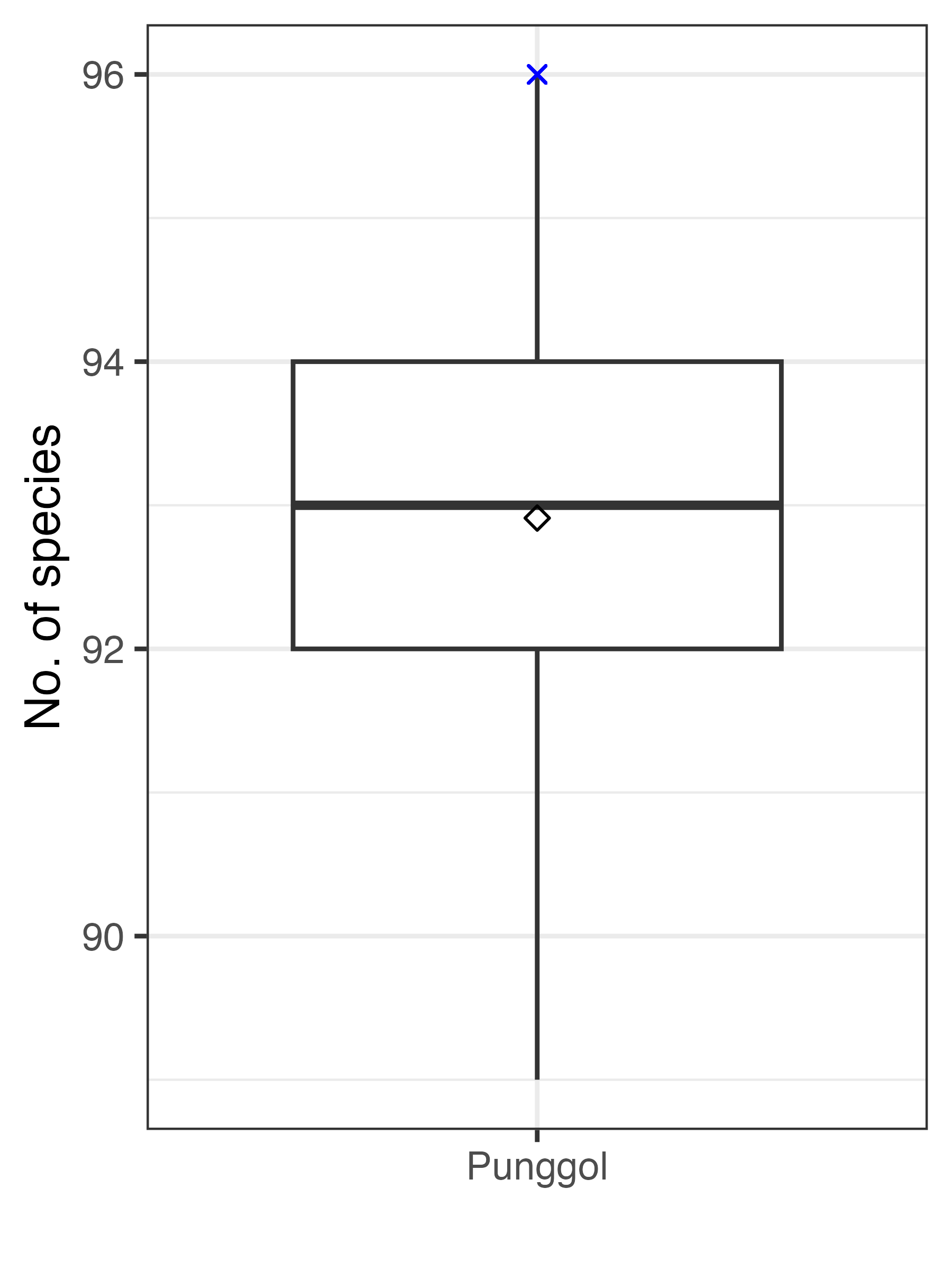

Figure: Number of bird species at Punggol, Singapore if 15 surveys were missed in Survey Cycle 5 (March – April 2017). The blue cross denotes the count in full dataset, while the diamond symbol denotes the mean count across 100 scenarios where survey data were randomly excluded.

Visualisations can also be performed at the level of individual species. Species that are relatively less common are more likely to be missed at sampling points:

# transform for plotting
plot_bird_spp <- scenarios %>%
  tidyr::pivot_longer(cols = num_range("iter", 1:ncol(scenarios)),
                      names_to = "iteration", values_to = "n") %>%
  dplyr::mutate(taxon = "Aves")

# get order of species based on total count
species_order <- plot_bird_spp %>%
  dplyr::group_by(species) %>%
  dplyr::summarise(order = mean(full))

plot_bird_spp %>%
  dplyr::left_join(species_order) %>% 
  ggplot(aes(x = reorder(species, order), y = n)) +
    geom_boxplot() +
    geom_point(aes(y = full), shape = 4, color = "blue") +
    stat_summary(fun = mean, geom = "point", shape = 5) + 
    xlab("") + ylab("No. of sampling points") + 
    theme_bw() +
    coord_flip()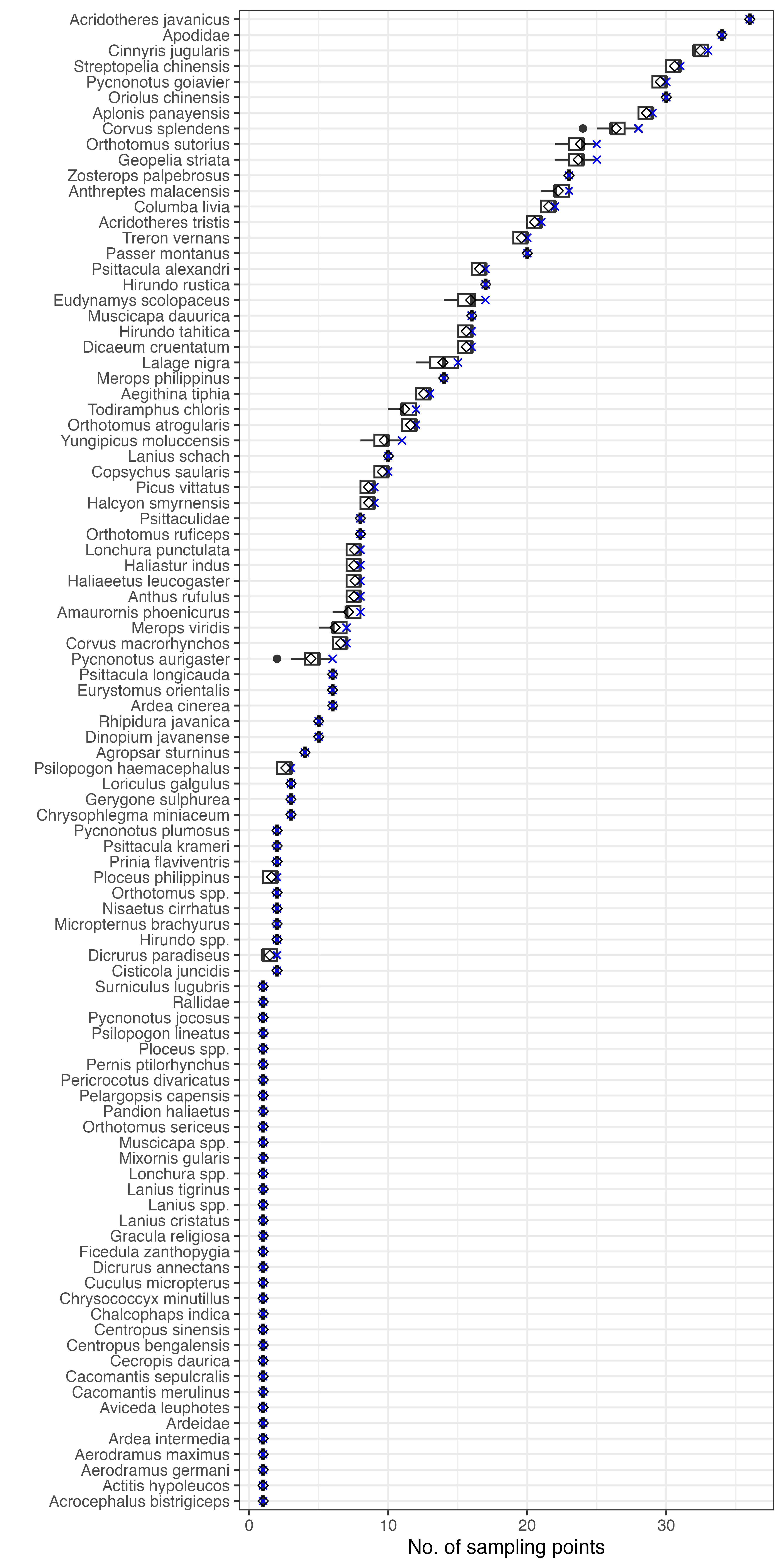 

Figure: Number of sampling points that bird species were observed at Punggol, Singapore if 15 surveys were missed in Survey Cycle 5 (March – April 2017). The blue cross denotes the count in full dataset, while the diamond symbol denotes the mean count across 100 scenarios where survey data were randomly excluded. Species are arranged in descending order of counts.