Animals: Species-level Analyses

Survey data for each animal (taxon) group can be summarised at multiple levels (e.g. area, period). For a particular animal group of interest, finer-grained summaries can also be generated—at the level of individual species. This article outlines how such summaries may be generated, using bird surveys conducted in Singapore as an example.

First, load the necessary packages to run the analysis:

library("biodivercity")
library("dplyr") # data processing
library("ggplot2") # data visualisation

Prepare data

Load the example data. Refer to help(animal_observations) and help(animal_surveys) for more details on these datasets.

data("animal_observations")
data("animal_surveys")

Show group-level (family/genus) observations where all species in the group are observed at each sampling point, using the function check_taxongrps(). These entries will later be removed at the respective points, in order to prevent over-counting the number of species. More details in vignette("process-animal").

remove <- check_taxongrps(animal_observations, level = "point")
remove

## # A tibble: 0 × 4
## # Groups:   point_id, period [0]
## # … with 4 variables: point_id <chr>, period <dbl>, name <chr>, n <int>

Most abundant species

Summarise the animal surveys based on how many individuals of each species are present at each sampling point. Tally the number of individuals per species, within each area, period and taxon:

plot_fauna <- animal_observations %>%
  group_by(species, area, period, taxon) %>% 
  summarise(count = sum(abundance)) %>% 
  mutate(area = factor(area, # re-arrange factors
                       levels = c("PG", "QT", "TP","JW", "BS", "WL")))
plot_fauna

## # A tibble: 1,664 × 5
## # Groups:   species, area, period [1,664]
##    species               area  period taxon   count
##    <chr>                 <fct>  <dbl> <chr>   <dbl>
##  1 Accipiter gularis     TP         2 Aves        1
##  2 Accipiter spp.        JW         2 Aves        1
##  3 Accipiter spp.        QT         2 Aves        1
##  4 Accipiter spp.        TP         2 Aves        2
##  5 Accipiter trivirgatus QT         1 Aves        1
##  6 Accipitriformes       PG         2 Aves        1
##  7 Accipitriformes       QT         2 Aves        1
##  8 Accipitriformes       TP         1 Aves        1
##  9 Acisoma panorpoides   BS         1 Odonata     1
## 10 Acisoma panorpoides   JW         2 Odonata    11
## # … with 1,654 more rows

The results can be visualised, for example, for bird species at the six areas (towns) in Singapore, across two survey periods:

# get the (descending) order of species to be plot
order  <- plot_fauna %>% 
  filter(taxon == "Aves") %>% # birds only
  group_by(species) %>%
  summarise(order = sum(count))

plot_fauna %>%
  filter(taxon == "Aves") %>% # birds only
  group_by(area, period) %>% # only plot top 10 species
  slice_max(count, n = 10) %>%
  left_join(order) %>% # get the order
  ggplot(aes(y = count, x = reorder(species, count))) +
    geom_col(width = 0.8, color = "black") +
    facet_grid(~ area + period) +
    ylab("Number of individuals") +
    xlab("")+
    theme_bw()+
    theme(text = element_text(size=8.0),
          axis.text.y = element_text(face = "italic"),
          panel.grid.major.y = element_blank(),
          panel.grid.minor.x = element_blank()) +
    coord_flip() +
    scale_y_continuous(expand = c(0,0), breaks = scales::breaks_pretty(n = 3))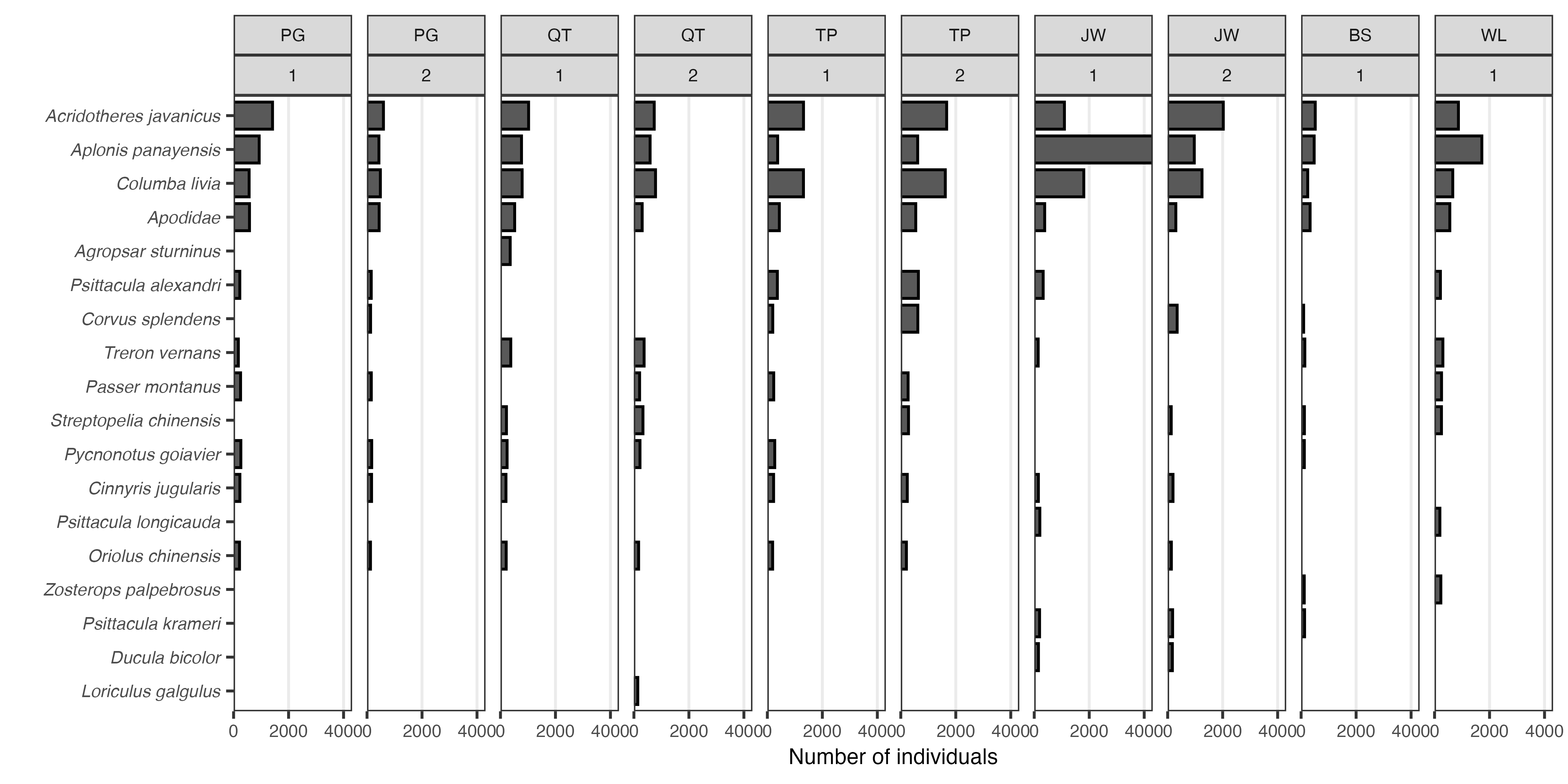

Figure: Most abundant bird species within each area (town), per survey round. Up to ten species are shown; species are arranged in descending order according to their cumulative counts.

Most common species

Summarise the animal surveys based on whether each species is present at sampling points. Tally the instances where each species is observed within each area, period, taxon and point_id:

plot_fauna <- animal_observations %>%
  group_by(species, area, period, taxon, point_id) %>% # counts of unique species at each sampling pt, per survey area/period/taxon
  summarise() %>% 
  anti_join(remove, by = c("species" = "name","point_id", "period")) %>% # exclude genus/family lvl records if all species within grp observed
  group_by(species, area, period, taxon) %>% # no. of points that each species occurs (per area/period/taxon)
  summarise(count = n()) %>% 
  mutate(area = factor(area, # re-arrange factors
                       levels = c("PG", "QT", "TP","JW", "BS", "WL")))

Similarly, common bird species within the six areas (towns) in Singapore can be visualised:

# get the (descending) order of species to be plot
order  <- plot_fauna %>% 
  filter(taxon == "Aves") %>% # birds only
  group_by(species) %>%
  summarise(order = sum(count))

plot_fauna %>%
  filter(taxon == "Aves") %>% # birds only
  group_by(area, period) %>% # only plot top 10 species 
  slice_max(count, n = 10) %>%
  left_join(order) %>% # get order
  ggplot(aes(y = count, x = reorder(species, order))) +
    geom_col(width = 0.8, color = "black") +
    facet_grid(~ area + period) +
    ylab("Number of sampling points") +
    xlab("")+
    theme_bw()+
    theme(text = element_text(size=8.0),
          axis.text.y = element_text(face = "italic"),
          panel.grid.major.y = element_blank(),
          panel.grid.minor.x = element_blank()) +
    coord_flip() +
    scale_y_continuous(expand = c(0,0), breaks = scales::breaks_pretty(n = 4))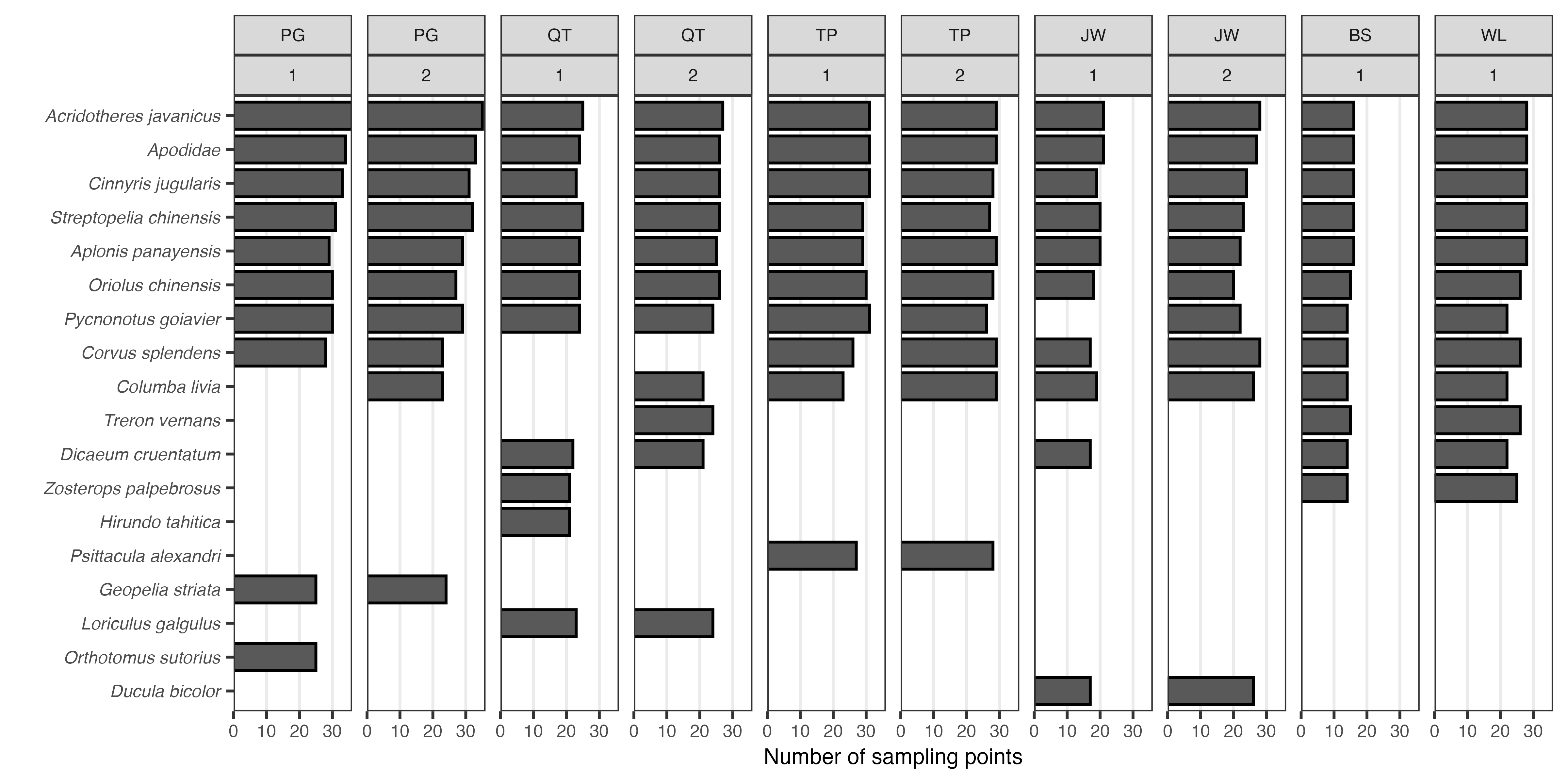

Figure: Most common bird species within each area (town), per survey round. Up to ten species are shown; species are arranged in descending order according to the cumulative number of sampling points they are present in.

More interesting visualisations can also be generated. For example, a hierarchical tree map may be used to show the ten most common bird species in the first survey period:

library(treemapify)

plot_fauna %>%
  filter(taxon == "Aves" & period == 1) %>% # birds in period 1 only
  group_by(area) %>% # only plot top 10 species
  slice_max(count, n = 10) %>% 
  ggplot(aes(area = count, fill = area, subgroup = species)) +
    geom_treemap() +
    geom_treemap_subgroup_border(color = "white", size = 7) +
    geom_treemap_subgroup_text(place = "centre", 
                               size = 16,
                               reflow = TRUE, # wrap text
                               fontface = "bold") +
  colorspace::scale_fill_discrete_qualitative("Harmonic") +
  labs(title="Urban birds of Singapore",
       caption="Most common spp. during surveys in 2016–2019",
       fill = NULL) +
  theme(aspect.ratio = 5/4,
        plot.title = element_text(hjust = 0.5, size = 30, face = "bold"),
        plot.caption = element_text(size = 12, face = "italic"),
        legend.position="bottom",
        legend.text = element_text(size = 12)) +
  guides(fill = guide_legend(nrow = 1))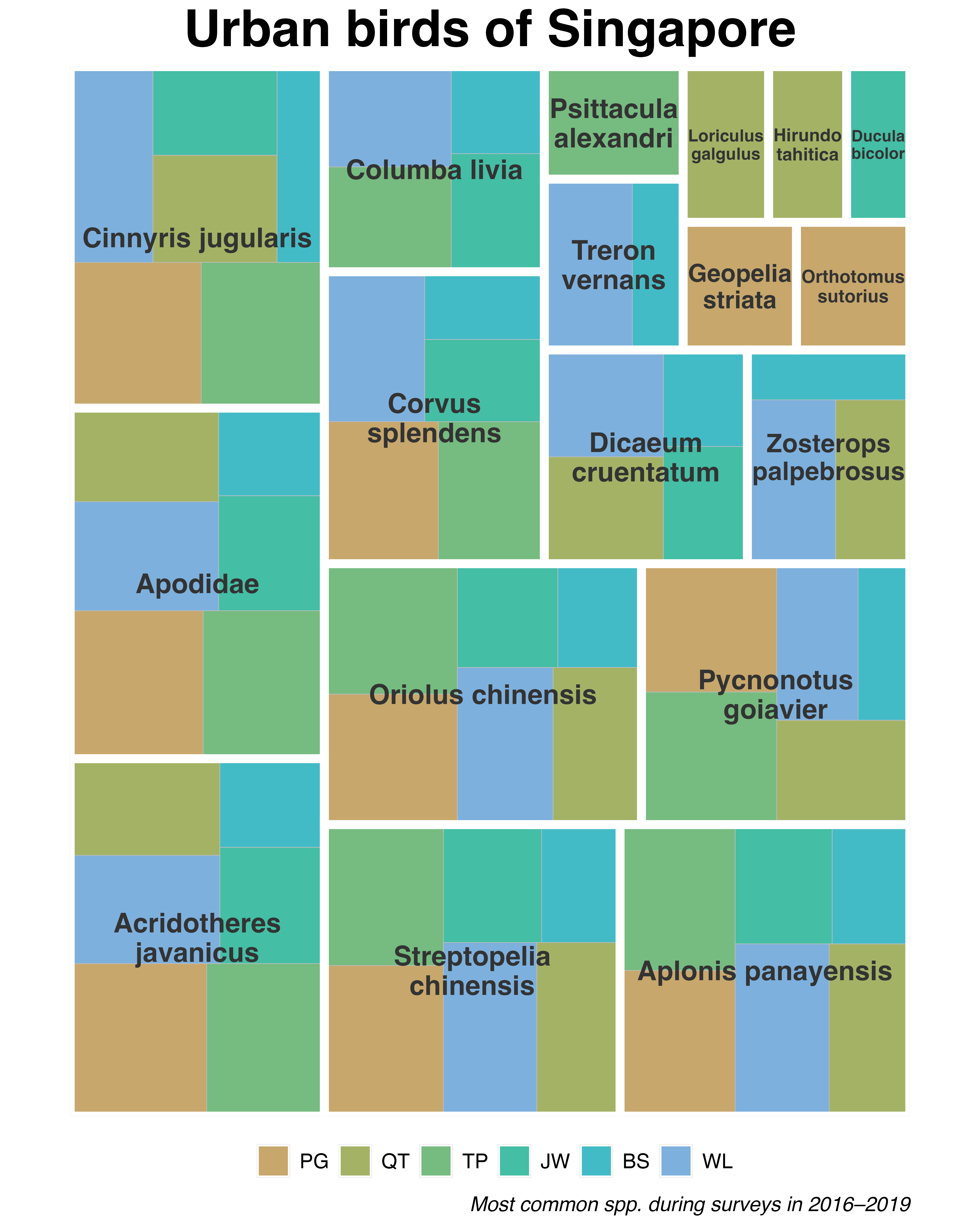

References

The latest accepted taxonomic names and local statuses in the example data are based on the following sources:

Birds: ebird Clements Checklist; The Singapore Red Data Book (Davison et al. 2008)
Butterflies: A Field Guide to the Butterflies of Singapore (Khew, 2010)
Odonates: The Dragonflies of Singapore: an updated checklist and revision of the national conservation statuses (Ngiam & Cheong, 2016)
Amphibians: A Guide to the Amphibians & Reptiles of Singapore (Lim & Lim, 2002)

Examine survey data at the level of individual species

2022-12-08

Prepare data

Most abundant species

Most common species

References