Animals: Survey Protocols
Systematically sample and record animal observations at point locations
2022-12-08
Source:vignettes/more/animals-survey-protocols.Rmd
animals-survey-protocols.RmdThis article describes a systematic way to conduct animal surveys, in order to collect a representative sample of data for a given area. The sampling strategy involves observations made at point locations (i.e. point surveys) for a fixed duration of time, within a fixed buffer radius from the point. The example data in this package were collected using the methods detailed here.
To begin, load the main libraries used in this analysis.
1. Pre-survey preparations
Generate new sampling points
Before surveys can begin, survey points have to be randomly generated within the area of interest. If necessary, stratified random sampling can be performed to ensure sufficient representation between sub-areas of interest.
Load the example data sampling_areas (sf polygons) for
six residential towns (areas) in Singapore, as well as patches of forest
cover sampling_forests that are within these towns
(sub-areas of interest). Note that forest cover for multiple Survey
Periods (see column name period) are present in
sampling_forests. Refer to
help(sampling_areas) and
help(sampling_forests) for more details.
head(sampling_areas)## Simple feature collection with 6 features and 1 field
## Geometry type: POLYGON
## Dimension: XY
## Bounding box: xmin: 353618.5 ymin: 141963.4 xmax: 384748.9 ymax: 161017.8
## Projected CRS: WGS 84 / UTM zone 48N
## area geometry
## 1 BS POLYGON ((371976.9 150656, ...
## 2 JW POLYGON ((358502.3 149045, ...
## 3 PG POLYGON ((379073.3 156986.3...
## 4 QT POLYGON ((365379.3 145134.7...
## 5 TP POLYGON ((384558.6 150112.5...
## 6 WL POLYGON ((363419.4 160258.2...
head(sampling_forests)## Simple feature collection with 6 features and 2 fields
## Geometry type: POLYGON
## Dimension: XY
## Bounding box: xmin: 364789.6 ymin: 141985.4 xmax: 366695.6 ymax: 145712.4
## Projected CRS: WGS 84 / UTM zone 48N
## area period geometry
## 1 QT 1 POLYGON ((364789.6 145712.4...
## 2 QT 1 POLYGON ((365541.3 144630.1...
## 3 QT 1 POLYGON ((365538.2 144603.3...
## 4 QT 1 POLYGON ((365992 142465.8, ...
## 5 QT 1 POLYGON ((365472.9 143750.2...
## 6 QT 1 POLYGON ((365615.5 143720.4...Using the area QT (Queenstown) as an example, sampling
points can be randomly generated. Subset both the example data to this
area, focusing on survey period 2.
queenstown <- sampling_areas[sampling_areas$area %in% "QT", ]
queenstown_forest <- sampling_forests[sampling_forests$area == "QT" & sampling_forests$period == 2,]
Next, within the area of interest, generate sampling points at a
specified density and buffer radius using the function
random_pt_gen(). In this case, we specify one point per 50
hectares (500000 m2), and a radius of 50 m for each point.
The radius value is the minimum distance between the generated points
and the boundaries—this ensures that the region for animal surveys does
not extend beyond the boundaries of Queenstown. An excess of sampling
points can be generated, in case some of these points are unsuitable for
surveys (e.g. within areas inaccessible to surveyors); for instance,
based on the specified parameters, 1.5 times the required
number points can be generated. Finally, sub-areas of interest
(queenstown_forest) can also be specified; sampling points
will be stratified between the areas within and
outside of queenstown_forest (i.e. ‘Forest’ and
‘Urban’ land cover types, respectively):
set.seed(123)

points <- random_pt_gen(boundaries = queenstown,
                        area_per_pt = 500000,
                        pt_radius = 50,
                        excess_modifier = 1.5,
                        sub_areas = queenstown_forest)
##
## Total number of points required: 13.
##
## Number of points required within 'normal' areas: 12.
## Number of points required within 'sub-areas': 1.
##
## Number of points within 'normal' areas that were generated: 18 (n = 12, excess_modifier = 1.5).
## Number of points within 'sub-areas' that were generated: 2 (n = 1, excess_modifier = 1.5).The output points is an sf object (POINT geometry)
containing the unique identifier, type (‘Normal’ or ‘Sub-area’) and
geographical coordinates for each point:
head(points)## Simple feature collection with 6 features and 2 fields
## Geometry type: POINT
## Dimension: XY
## Bounding box: xmin: 364719 ymin: 142645.6 xmax: 367118.5 ymax: 143706.5
## Projected CRS: WGS 84 / UTM zone 48N
## type id x
## 1 Normal normal1 POINT (366618 142645.6)
## 2 Normal normal2 POINT (366155.9 142805.7)
## 3 Normal normal3 POINT (365832.6 143706.5)
## 4 Normal normal4 POINT (367118.5 142757.4)
## 5 Normal normal5 POINT (364719 143528.1)
## 6 Normal normal6 POINT (366407.7 142761.1)Visualise the generated points within queenstown:
ggplot(data = queenstown) +
  geom_sf(fill = NA) +
  theme_void() +
  geom_sf(data = queenstown_forest, fill = "darkgreen") +
  geom_sf(data = points, aes(col = type),
          show.legend = "point")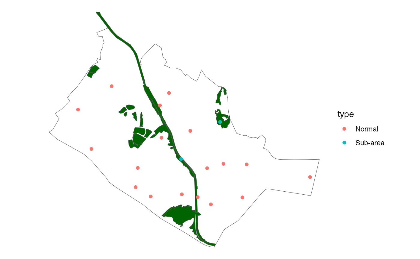
Retain sampling points
If surveys are conducted across multiple periods (e.g. years), there
may be a need to retain sampling points from a previous period, for
example, for long-term monitoring at the same location. If this is the
case, new points can be generated while ensuring that a certain
proportion of these points are similar to those from a previous period.
Note that the column type must also exist in the old
dataset, with the value of either Normal or
Sub-area. For example, we can choose to retain points in
Queenstown from Survey Period 1, which we assign to the
variable queenstown_retain:
data(sampling_points)
queenstown_retain <- sampling_points[sampling_points$area %in% "QT" & sampling_points$period %in% "1", ]

# create column 'type', which is based on the column 'landcover' in this example data
queenstown_retain <- queenstown_retain %>%
  mutate(type = ifelse(landcover == "Urban", "Normal", "Sub-area"))
If we wish to retain half of the points, add
queenstown_retain to the function argument
‘retain’, and set the argument ‘retain_prop’
to 0.5:
points <- random_pt_gen(boundaries = queenstown,
                        area_per_pt = 500000,
                        pt_radius = 50,
                        excess_modifier = 1.5,
                        sub_areas = queenstown_forest,
                        retain = queenstown_retain,
                        retain_prop = 0.5)
##
## Total number of points required: 13.
##
## Number of points required within 'normal' areas: 12.
## Number of points required within 'sub-areas': 1.
##
## Number of points within 'normal' areas that were retained: 6 (n = 12, retain_prop = 0.5).
## Number of points within 'sub-areas' that were retained: 1 (n = 1, retain_prop = 0.5).
## Number of new points within 'normal' areas that were generated: 9 (n = 6, excess_modifier = 1.5).
## Number of new points within 'sub-areas' that were generated: 1 (n = 0.5, excess_modifier = 1.5).If there were points that were retained, the additional column
‘status’ indicates whether the points generated are
‘Old’ or ‘New’.
head(points)## Simple feature collection with 6 features and 3 fields
## Geometry type: POINT
## Dimension: XY
## Bounding box: xmin: 365267.7 ymin: 142299.4 xmax: 368232.5 ymax: 145167
## Projected CRS: WGS 84 / UTM zone 48N
## id status type geometry
## 1 normal1 New Normal POINT (366281.2 142299.4)
## 2 normal2 New Normal POINT (368232.5 143131.8)
## 3 normal3 New Normal POINT (365983.4 143815.4)
## 4 normal4 New Normal POINT (365267.7 145167)
## 5 normal5 New Normal POINT (365277.3 144234.9)
## 6 normal6 New Normal POINT (367253.4 143360.6)
ggplot(data = queenstown) +
  geom_sf(fill = NA) +
  theme_void() +
  geom_sf(data = queenstown_forest, fill = "darkgreen") +
  geom_sf(data = points,
          aes(col = type, shape = status))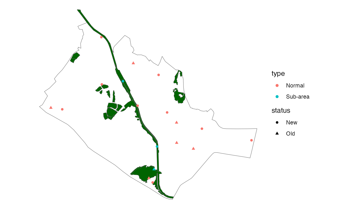
Finally, surveyors can proceed to assess the sampling points and
their surrounding areas (up to the buffer radius, e.g., 50 m). Factors
to take note of include (1) accessibility; (2) potential disturbance to
wild animals (e.g. nearby construction). To ensure that random sampling
is maintained, suitable points should be selected according to the order
in which they were generated (the column id).
2. Animal surveys
Data format
Animal survey data are organised into two separate tables, shown below.
| survey_id | point_id | area | period | cycle | resampled | start_time | time | taxon | species | family | genus | abundance |
|---|---|---|---|---|---|---|---|---|---|---|---|---|
| 1 QTNa14a_P 1 Odonata | QTNa14a_P | QT | 1 | 1 | NA | 2016-08-04 14:00:00 | 2016-08-04 14:01:00 | Odonata | Rhyothemis phyllis | Libellulidae | Rhyothemis spp. | 3 |
| 1 QTNa14a_P 1 Odonata | QTNa14a_P | QT | 1 | 1 | NA | 2016-08-04 14:00:00 | 2016-08-04 14:12:00 | Odonata | Crocothemis servilia | Libellulidae | Crocothemis spp. | 1 |
| 1 QTNa14a_P 1 Odonata | QTNa14a_P | QT | 1 | 1 | NA | 2016-08-04 14:00:00 | 2016-08-04 14:15:00 | Odonata | Neurothemis fluctuans | Libellulidae | Neurothemis spp. | 1 |
| 1 QTNa14a_P 1 Odonata | QTNa14a_P | QT | 1 | 1 | NA | 2016-08-04 14:00:00 | 2016-08-04 14:23:00 | Odonata | Crocothemis servilia | Libellulidae | Crocothemis spp. | 1 |
| 1 QTNa14a_P 1 Odonata | QTNa14a_P | QT | 1 | 1 | NA | 2016-08-04 14:00:00 | 2016-08-04 14:28:00 | Odonata | Neurothemis fluctuans | Libellulidae | Neurothemis spp. | 1 |
| 1 QTNb1a_P 1 Odonata | QTNb1a_P | QT | 1 | 1 | NA | 2016-08-04 14:44:00 | 2016-08-04 14:44:00 | Odonata | Neurothemis fluctuans | Libellulidae | Neurothemis spp. | 1 |
| survey_id | point_id | area | period | cycle | taxon | resampled | start_time | notes |
|---|---|---|---|---|---|---|---|---|
| 1 QTNa14a_P 1 Odonata | QTNa14a_P | QT | 1 | 1 | Odonata | NA | 2016-08-04 14:00:00 | NA |
| 1 QTNb1a_P 1 Odonata | QTNb1a_P | QT | 1 | 1 | Odonata | NA | 2016-08-04 14:44:00 | NA |
| 1 QTNa14a_P 1 Amphibia | QTNa14a_P | QT | 1 | 1 | Amphibia | NA | 2016-08-04 19:55:00 | NA |
| 1 QTNb1a_P 1 Amphibia | QTNb1a_P | QT | 1 | 1 | Amphibia | NA | 2016-08-04 20:40:00 | NA |
| 1 PGT15 1 Aves | PGT15 | PG | 1 | 1 | Aves | NA | 2016-08-08 07:00:00 | NA |
| 1 PGT14 1 Aves | PGT14 | PG | 1 | 1 | Aves | NA | 2016-08-08 07:33:00 | NA |
Data collection
In the example datasets animal_observations and
animal_surveys, 30-minute surveys were conducted within the
designated buffer radius for the specific animal (taxon) group. For
example, the buffer radius for Bird (Aves) surveys is 50 m, while those
for Butterflies (Lepidoptera), Odonates (Odonata) and Amphibians
(Amphibia) are at 20 m from the sampling point location. The survey time
window also varies for each animal group, and were chosen based on
previous research. In addition, Odonate and Amphibian surveys conducted
at sampling points with ephemeral water bodies had to be performed
within 24 hours after a rain event. The rain event had to be of at least
a light–moderate intensity, based on real-time
updates from Meteorological Service Singapore.
| Taxon | Time | Radius (m) |
|---|---|---|
| Birds | 0700–0930 | 50 |
| Butterflies | 0930–1200 | 20 |
| Odonates | 1400–1600 | 20 |
| Amphibians | 2000–2200 | 20 |
Surveyors move within the buffer radius to identify and count the
number of species. Each encounter is recorded according to individual
species; information about the time, abundance and distance from the
center point are also recorded. Refer to
help(animal_observations) for more information.
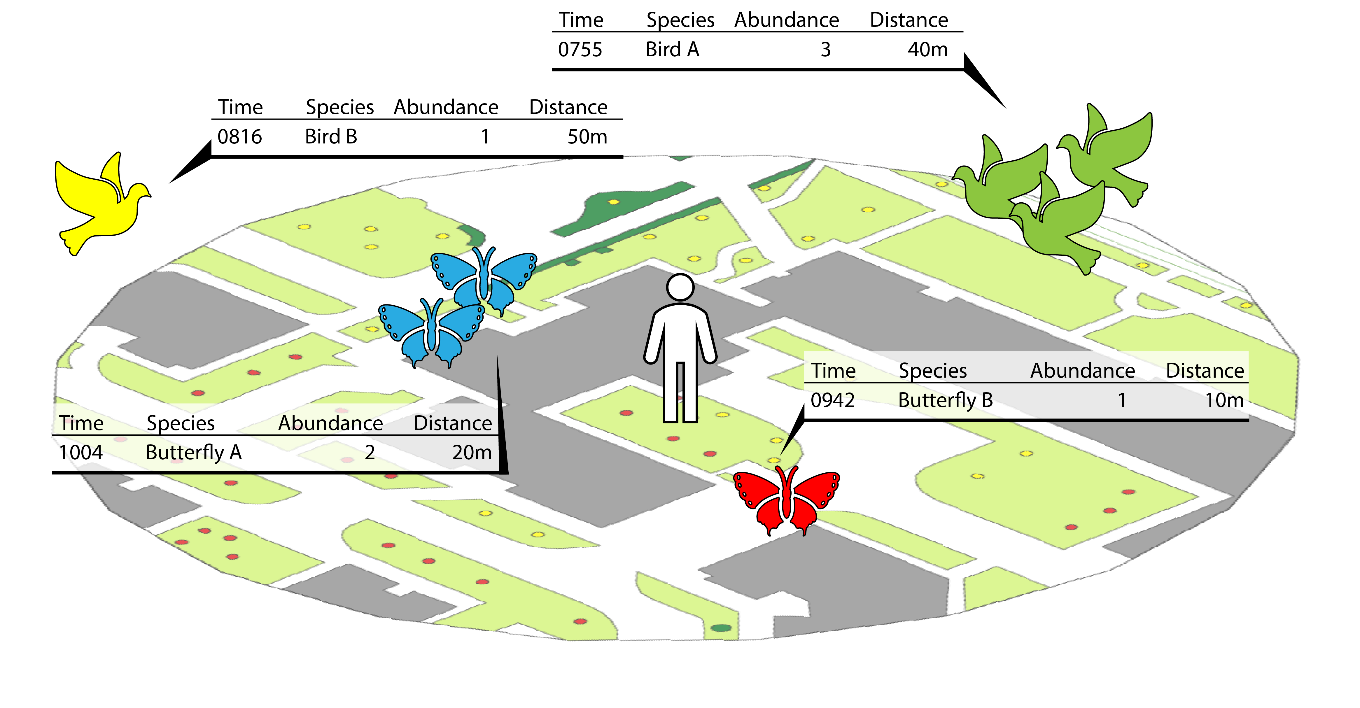
Figure: Example showing the information recorded for animal observations from the surveyor’s point-of-view.
Sampling points were surveyed once every two months
(cycle adds up to six per survey period); each
sampling period thus stretched across a year-long duration.