Process Landscape Data
Download and summarise landscape data at point locations
2022-12-08
Source:vignettes/process-landscape.Rmd
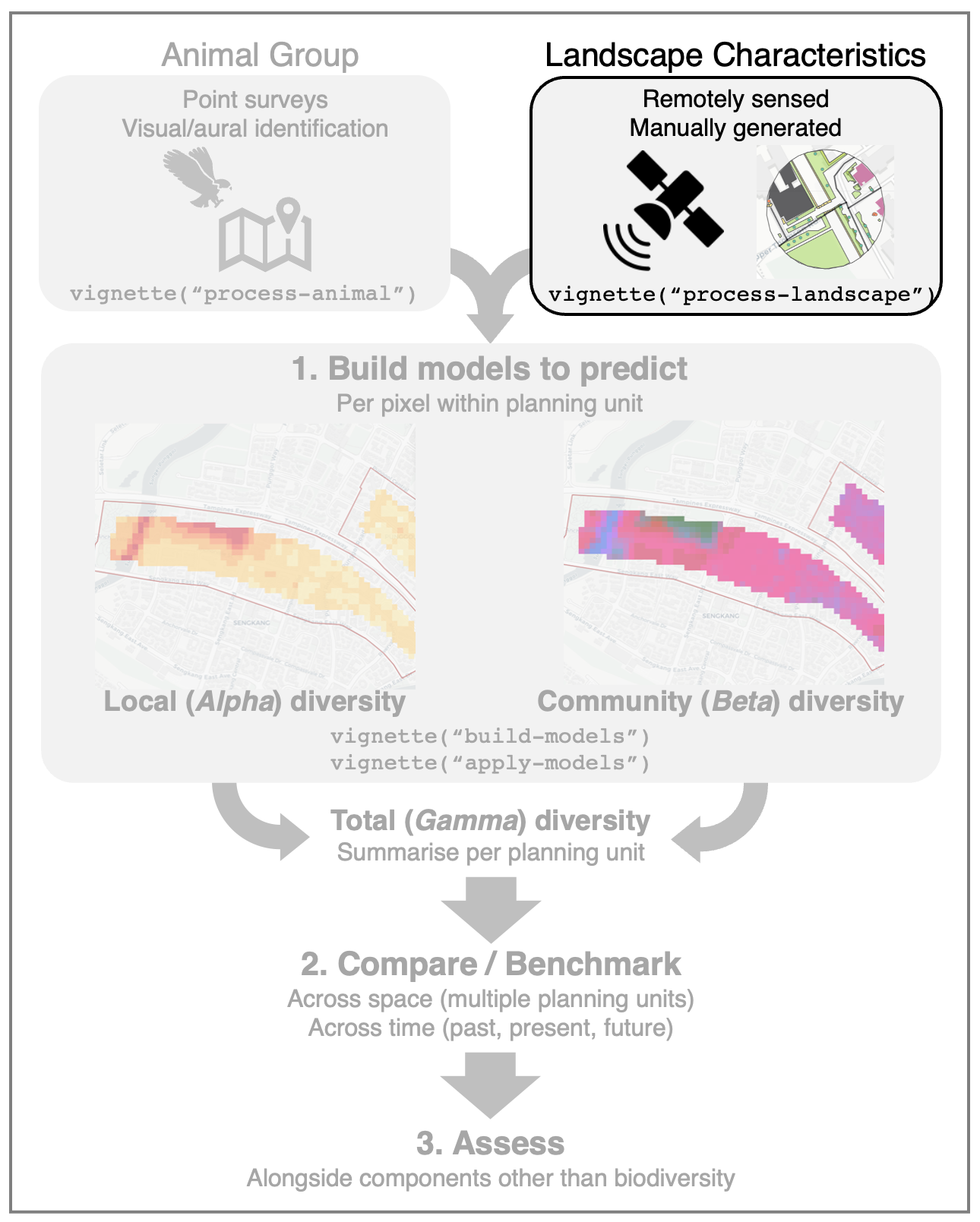
process-landscape.RmdThis article details various ways to download and process landscape data to build predictive models of animal diversity. For example, the landscape data may be derived from (1) remotely sensed satellite imagery, (2) open-source maps, or (3) manually generated sources (e.g., from on-site mapping, design scenarios). We give examples of each in this article.
First, load the necessary packages to run the analysis:
library("biodivercity")
library("dplyr") # to process/wrangle data
library("sf") # to process vector data
library("tmap") # for visualisationNext, define an output directory for raw and processed data to be exported to:
output_dir <- "</FILEPATH/TO/DIRECTORY>"In this article, the Punggol (PG) area in Singapore from
the example dataset sampling_areas will be used. Landscape
data can be summarised at point locations where animal data are
available (e.g., animal surveys have been conducted); to demonstrate
this, we randomly generate three points within Punggol and assign it to
the object ‘points’:
data(sampling_areas)
sampling_areas <- sampling_areas %>%
filter(area == "PG")
# randomly generate 3 points
set.seed(30)
points <- st_sample(sampling_areas, 3) %>%
st_as_sf() %>%
mutate(point_id = row.names(.)) # unique identifier
tmap_mode("view")
tm_basemap(c("CartoDB.Positron")) +
tm_shape(sampling_areas) + tm_borders() +
tm_shape(points) + tm_dots()1. Remotely sensed land cover
Land cover can be a useful predictor of animal diversity. For
example, publicly-available data from Sentinel-2 may be downloaded using
the package sen2r.
The package includes data pre-processing steps such as cloud masking,
atmospheric correction and the calculation of spectral indices.
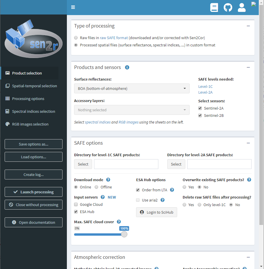
Figure: A screenshot of the sen2r graphical user
interface accessible by running sen2r::sen2r().
Data processing parameters can be specified as arguments within
sen2r(), or loaded from a JSON file. In the example below,
we download data from 1 Jan to 30 Jun 2021, with not more than 15% cloud
cover within sampling_areas. For each image, the spectral
indices NDVI
and NDWI2
are processed; these will be used to map vegetation and water cover,
respectively. Do note that you will need to enter your account
credentials for the ESA Sentinel Hub.
Detailed steps and the use of other servers (e.g. Google Cloud) can be
found in the package
website.
# create sub-directories
dir.create(paste0(output_dir, "/sen2r")) # for processed output files
dir.create(paste0(output_dir, "/sen2r/raw")) # for raw files
# execute workflow
out_paths <- sen2r(
timewindow = as.Date(c("2021-01-01", "2021-06-30")),
max_cloud_safe = 15, # max 15% cloud cover in raw tile
max_mask = 15, # max 15% cloud cover over sampling_areas
extent = geojsonsf::sf_geojson(sampling_areas) # needs geojson as input
clip_on_extent = TRUE,
list_indices = c("NDVI", "NDWI2") # to map vegetation and water
list_rgb = "RGB432B", # output an RGB image as well
path_l2a = paste0(output_dir, "/sen2r/raw"),
path_l1c = paste0(output_dir, "/sen2r/raw"),
path_out = paste0(output_dir, "/sen2r"),
path_indices = paste0(output_dir, "/sen2r"))For each spectral index, we can combine all raster images captured
within the specified date range by averaging the pixel values across
files, thus forming an image mosaic. This allows us to avoid relying on
any one image for our analysis, and to deal with missing data (e.g. due
to high cloud cover) during the period of interest. The function
mosaic_sen2r() creates the mosaic by averaging the pixel
values across the multiple rasters. It is a convenience function that
processes the images based on the output folder structure of
sen2r(); ensure that the function argument
parent_dir in mosaic_sen2r() is similar to the
function argument path_out in sen2r().
mosaic_sen2r(parent_dir = paste0(output_dir, "/sen2r"))At this point, we have a single image mosaic (continuous raster) for
each spectral index, for a given area/period of interest. While the
continuous values from these rasters may be used directly in analyses,
there may be instances were we want to work with discrete classes of
land cover. To do so, we can classify pixels into one of two classes
(e.g. vegetated or non-vegetated; water or non-water), based on an
adaptively derived threshold value. For example, we can use Otsu’s
thresholding (Otsu,
1979), which tends to outperform other techniques in terms of
stability of results and processing speed, even with the presence of
> 2 peaks in the histogram of pixel values (Bouhennache
et al., 2019). This can be implemented using the function
threshold_otsu(). As an example, let’s load the NDVI raster
for the Punggol area in Singapore for subsequent classification. The
NDVI is a measure of healthy green vegetation, based on the tendency of
plants to reflect NIR & absorb red light. It ranges from -1
(non-vegetated) to 1 (densely vegetated). The figure below shows the
histogram of NDVI values within Punggol, as well as the adaptively
derived threshold value (vertical line).
ndvi_mosaic <-
system.file("extdata", "ndvi_mosaic.tif", package="biodivercity") %>%
terra::rast()
# get Otsu's threshold
threshold <- threshold_otsu(ndvi_mosaic)
threshold## [1] 0.3945684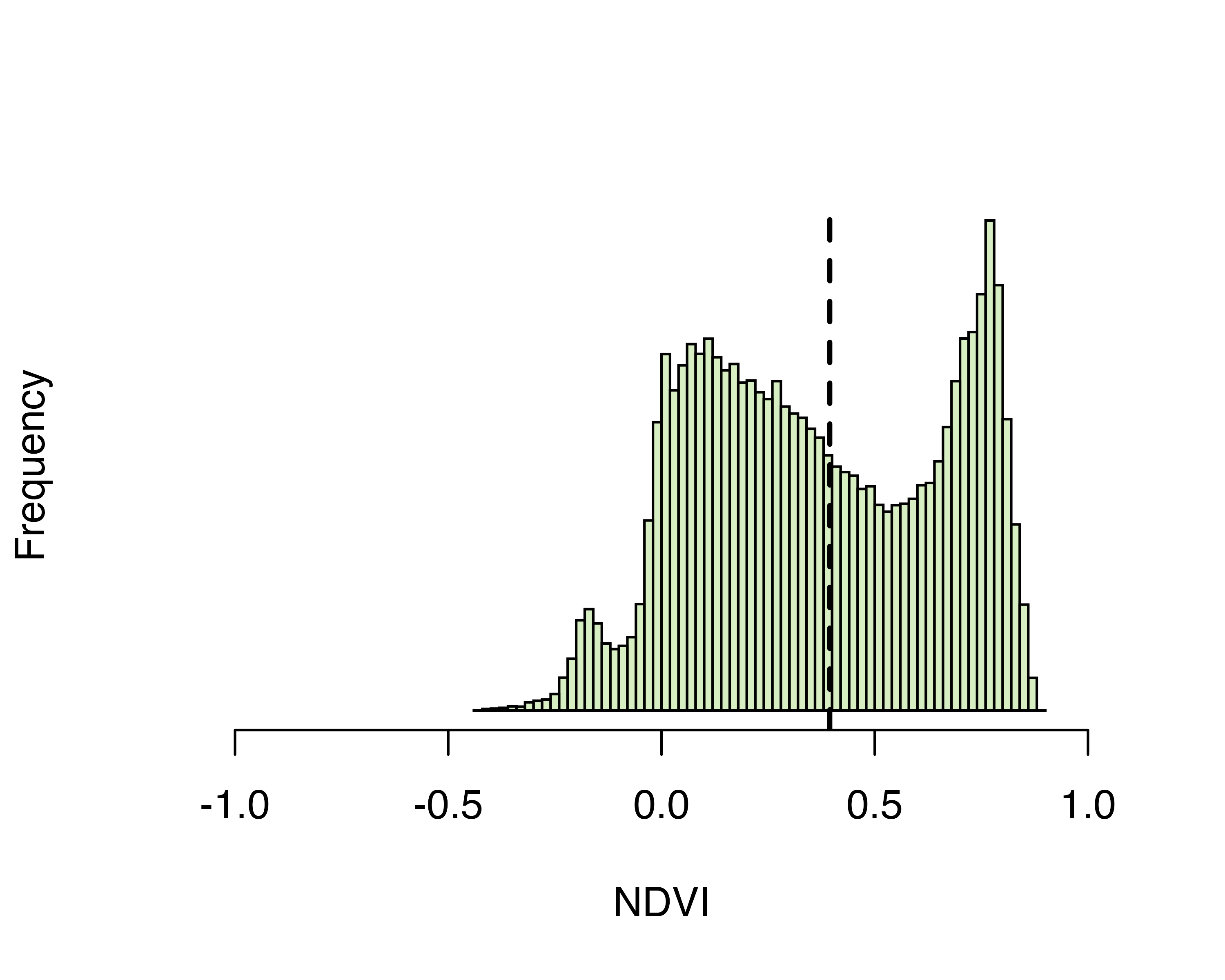
Figure: Distribution of NDVI values across the Punggol area in Singapore, based on a mosaic of images collected from 2019-07-01 to 2021-06-30. Pixel values to the right of the dashed line may be classified as ‘vegetated’, while those to the left are ‘non-vegetated’.
The function classify_image_binary() can be used to
directly classify a continuous raster (e.g., image mosaic). Note that it
uses threshold_otsu() internally to define the threshold
value. See the map below to examine both the original NDVI and
classified rasters within the Punggol area in Singapore (toggle the map
layers to view each one separately).
veg_classified <- classify_image_binary(ndvi_mosaic, threshold = "otsu")
tm_basemap(c("CartoDB.Positron")) +
tm_shape(ndvi_mosaic) +
tm_raster(palette = c("Greens")) +
tm_shape(veg_classified) +
tm_raster(style = "cat",
palette = c("grey", "darkgreen")) +
tm_shape(points) + tm_dots()‘Landscape metrics’ can then be used to represent the composition and spatial patterns of land cover within the area of interest. For each classified raster, metrics can be summarised at specific point locations and at multiple buffer radii. Metrics can also be calculated at various ‘levels’, or unit of analysis — patch, class, and landscape (in order of widening spatial scale). Refer to the package landscapemetrics for more information.
| metric | name | type | class | landscape |
|---|---|---|---|---|
| ai | aggregation index | aggregation metric | Yes | Yes |
| area_cv | patch area (coef. of variation) | area and edge metric | Yes | Yes |
| area_mn | patch area (mean) | area and edge metric | Yes | Yes |
| area_sd | patch area (st. dev.) | area and edge metric | Yes | Yes |
| cai_cv | core area index (coef. of variation) | core area metric | Yes | Yes |
| cai_mn | core area index (mean) | core area metric | Yes | Yes |
| cai_sd | core area index (st. dev.) | core area metric | Yes | Yes |
| circle_cv | related circumscribing circle (coef. of variation) | shape metric | Yes | Yes |
| circle_mn | related circumscribing circle (mean) | shape metric | Yes | Yes |
| circle_sd | related circumscribing circle (st. dev.) | shape metric | Yes | Yes |
| cohesion | patch cohesion index | aggregation metric | Yes | Yes |
| contig_cv | contiguity index (coef. of variation) | shape metric | Yes | Yes |
| contig_mn | contiguity index (mean) | shape metric | Yes | Yes |
| contig_sd | contiguity index (st. dev.) | shape metric | Yes | Yes |
| core_cv | core area (coef. of variation) | core area metric | Yes | Yes |
| core_mn | core area (mean) | core area metric | Yes | Yes |
| core_sd | core area (st. dev.) | core area metric | Yes | Yes |
| dcad | disjunct core area density | core area metric | Yes | Yes |
| dcore_cv | disjunct core area (coef. of variation) | core area metric | Yes | Yes |
| dcore_mn | disjunct core area (mean) | core area metric | Yes | Yes |
| dcore_sd | disjunct core area (st. dev.) | core area metric | Yes | Yes |
| division | division index | aggregation metric | Yes | Yes |
| ed | edge density | area and edge metric | Yes | Yes |
| enn_cv | euclidean nearest neighbor distance (coef. of variation) | aggregation metric | Yes | Yes |
| enn_mn | euclidean nearest neighbor distance (mean) | aggregation metric | Yes | Yes |
| enn_sd | euclidean nearest neighbor distance (st. dev.) | aggregation metric | Yes | Yes |
| frac_cv | fractal dimension index (coef. of variation) | shape metric | Yes | Yes |
| frac_mn | fractal dimension index (mean) | shape metric | Yes | Yes |
| frac_sd | fractal dimension index (st. dev.) | shape metric | Yes | Yes |
| gyrate_cv | radius of gyration (coef. of variation) | area and edge metric | Yes | Yes |
| gyrate_mn | radius of gyration (mean) | area and edge metric | Yes | Yes |
| gyrate_sd | radius of gyration (st. dev.) | area and edge metric | Yes | Yes |
| iji | interspersion and juxtaposition index | aggregation metric | Yes | Yes |
| lpi | largest patch index | area and edge metric | Yes | Yes |
| lsi | landscape shape index | aggregation metric | Yes | Yes |
| mesh | effective mesh size | aggregation metric | Yes | Yes |
| ndca | number of disjunct core areas | core area metric | Yes | Yes |
| np | number of patches | aggregation metric | Yes | Yes |
| pafrac | perimeter-area fractal dimension | shape metric | Yes | Yes |
| para_cv | perimeter-area ratio (coef. of variation) | shape metric | Yes | Yes |
| para_mn | perimeter-area ratio (mean) | shape metric | Yes | Yes |
| para_sd | perimeter-area ratio (st. dev.) | shape metric | Yes | Yes |
| pd | patch density | aggregation metric | Yes | Yes |
| pladj | percentage of like adjacencies | aggregation metric | Yes | Yes |
| shape_cv | shape index (coef. of variation) | shape metric | Yes | Yes |
| shape_mn | shape index (mean) | shape metric | Yes | Yes |
| shape_sd | shape index (st. dev.) | shape metric | Yes | Yes |
| split | splitting index | aggregation metric | Yes | Yes |
| tca | total core area | core area metric | Yes | Yes |
| te | total edge | area and edge metric | Yes | Yes |
| ca | total (class) area | area and edge metric | Yes | No |
| clumpy | clumpiness index | aggregation metric | Yes | No |
| cpland | core area percentage of landscape | core area metric | Yes | No |
| nlsi | normalized landscape shape index | aggregation metric | Yes | No |
| pland | percentage of landscape | area and edge metric | Yes | No |
| condent | conditional entropy | complexity metric | No | Yes |
| contag | connectance | aggregation metric | No | Yes |
| ent | shannon entropy | complexity metric | No | Yes |
| joinent | joint entropy | complexity metric | No | Yes |
| msidi | modified simpson’s diversity index | diversity metric | No | Yes |
| msiei | modified simpson’s evenness index | diversity metric | No | Yes |
| mutinf | mutual information | complexity metric | No | Yes |
| pr | patch richness | diversity metric | No | Yes |
| prd | patch richness density | diversity metric | No | Yes |
| relmutinf | relative mutual information | complexity metric | No | Yes |
| shdi | shannon’s diversity index | diversity metric | No | Yes |
| shei | shannon’s evenness index | diversity metric | No | Yes |
| sidi | simpson’s diversity index | diversity metric | No | Yes |
| siei | simspon’s evenness index | diversity metric | No | Yes |
A wide variety of landscape metrics can be summarised at point
locations of interest, using the function calc_lsm(). The
following example summarises all ‘class-level’ metrics for vegetation
cover (veg_classified), up to 200 and
400 metres away from points. This returns a
list, with each element corresponding to a particular buffer radius.
Column names include a prefix indicating that values are landscape
metrics derived from a classified raster (lsm_).
lsm_perpoint <-
calc_lsm(raster = veg_classified,
points = points,
buffer_sizes = c(200, 400), # in metres
level = c("class"),
class_names = c("veg"), # land cover class name
class_values = c(1)) # pixel value of class
lsm_perpoint## $`200`
## # A tibble: 3 × 57
## point_id percentage_…¹ lsm_v…² lsm_v…³ lsm_v…⁴ lsm_v…⁵ lsm_v…⁶ lsm_v…⁷ lsm_v…⁸
## <chr> <dbl> <dbl> <dbl> <dbl> <dbl> <dbl> <dbl> <dbl>
## 1 1 80.0 72.6 299. 0.169 0.505 2.87 229. 4.95
## 2 2 99.9 68.4 169. 0.183 0.309 3.47 175. 6.33
## 3 3 100. 74.7 157. 0.264 0.415 3.17 154. 12.2
## # … with 48 more variables: lsm_veg_cai_sd <dbl>, lsm_veg_circle_cv <dbl>,
## # lsm_veg_circle_mn <dbl>, lsm_veg_circle_sd <dbl>, lsm_veg_clumpy <dbl>,
## # lsm_veg_cohesion <dbl>, lsm_veg_contig_cv <dbl>, lsm_veg_contig_mn <dbl>,
## # lsm_veg_contig_sd <dbl>, lsm_veg_core_cv <dbl>, lsm_veg_core_mn <dbl>,
## # lsm_veg_core_sd <dbl>, lsm_veg_cpland <dbl>, lsm_veg_dcad <dbl>,
## # lsm_veg_dcore_cv <dbl>, lsm_veg_dcore_mn <dbl>, lsm_veg_dcore_sd <dbl>,
## # lsm_veg_division <dbl>, lsm_veg_ed <dbl>, lsm_veg_enn_cv <dbl>, …
##
## $`400`
## # A tibble: 3 × 57
## point_id percentage_…¹ lsm_v…² lsm_v…³ lsm_v…⁴ lsm_v…⁵ lsm_v…⁶ lsm_v…⁷ lsm_v…⁸
## <chr> <dbl> <dbl> <dbl> <dbl> <dbl> <dbl> <dbl> <dbl>
## 1 1 66.7 74.8 363. 0.302 1.10 11.5 191. 6.34
## 2 2 99.1 77.0 318. 0.339 1.08 17.6 209. 6.95
## 3 3 97.0 78.0 379. 0.301 1.14 15.1 183. 7.35
## # … with 48 more variables: lsm_veg_cai_sd <dbl>, lsm_veg_circle_cv <dbl>,
## # lsm_veg_circle_mn <dbl>, lsm_veg_circle_sd <dbl>, lsm_veg_clumpy <dbl>,
## # lsm_veg_cohesion <dbl>, lsm_veg_contig_cv <dbl>, lsm_veg_contig_mn <dbl>,
## # lsm_veg_contig_sd <dbl>, lsm_veg_core_cv <dbl>, lsm_veg_core_mn <dbl>,
## # lsm_veg_core_sd <dbl>, lsm_veg_cpland <dbl>, lsm_veg_dcad <dbl>,
## # lsm_veg_dcore_cv <dbl>, lsm_veg_dcore_mn <dbl>, lsm_veg_dcore_sd <dbl>,
## # lsm_veg_division <dbl>, lsm_veg_ed <dbl>, lsm_veg_enn_cv <dbl>, …This list object can then be converted into a dataframe, with a new column indicating the radii in which these landscape metrics have been summarised.
## # A tibble: 6 × 58
## radius point…¹ perce…² lsm_v…³ lsm_v…⁴ lsm_v…⁵ lsm_v…⁶ lsm_v…⁷ lsm_v…⁸ lsm_v…⁹
## <chr> <chr> <dbl> <dbl> <dbl> <dbl> <dbl> <dbl> <dbl> <dbl>
## 1 200 1 80.0 72.6 299. 0.169 0.505 2.87 229. 4.95
## 2 200 2 99.9 68.4 169. 0.183 0.309 3.47 175. 6.33
## 3 200 3 100. 74.7 157. 0.264 0.415 3.17 154. 12.2
## 4 400 1 66.7 74.8 363. 0.302 1.10 11.5 191. 6.34
## 5 400 2 99.1 77.0 318. 0.339 1.08 17.6 209. 6.95
## 6 400 3 97.0 78.0 379. 0.301 1.14 15.1 183. 7.35
## # … with 48 more variables: lsm_veg_cai_sd <dbl>, lsm_veg_circle_cv <dbl>,
## # lsm_veg_circle_mn <dbl>, lsm_veg_circle_sd <dbl>, lsm_veg_clumpy <dbl>,
## # lsm_veg_cohesion <dbl>, lsm_veg_contig_cv <dbl>, lsm_veg_contig_mn <dbl>,
## # lsm_veg_contig_sd <dbl>, lsm_veg_core_cv <dbl>, lsm_veg_core_mn <dbl>,
## # lsm_veg_core_sd <dbl>, lsm_veg_cpland <dbl>, lsm_veg_dcad <dbl>,
## # lsm_veg_dcore_cv <dbl>, lsm_veg_dcore_mn <dbl>, lsm_veg_dcore_sd <dbl>,
## # lsm_veg_division <dbl>, lsm_veg_ed <dbl>, lsm_veg_enn_cv <dbl>, …2. OpenStreetMap landscape elements
Landscape elements can be retrieved from the open-source maps such as
OpenStreetMap (OSM). For instance, built elements such as building
polygons and road lines can be extracted from
sampling_areas using the functions
get_buildings_osm() and get_roads_osm(),
respectively. The date argument, if specified, must be a
snapshot date present within the Geofabrik database. If not, the
latest data will be downloaded. In this example, we download these urban
elements for the date 1 Jan 2021 and view them as an interactive
map:
dir.create(paste0(output_dir, "/osm")) # create sub-directory for raw data (avoid re-downloading each time)
buildings_osm <- get_buildings_osm(place = sampling_areas,
date = as.Date("2021-01-01"),
dir_raw = paste0(output_dir, "/osm"))
roads_osm <- get_roads_osm(sampling_areas,
date = as.Date("2021-01-01"),
dir_raw = paste0(output_dir, "/osm"))
# alternatively, load example dataset from package
filepath <- system.file("extdata", "osm_data.Rdata", package = "biodivercity")
load(filepath)
# plot
tm_basemap(c("CartoDB.Positron")) +
tm_shape(sampling_areas) + tm_borders() +
tm_shape(buildings_osm) + tm_polygons(col = "levels") +
tm_shape(roads_osm) + tm_lines(col = "lanes", palette = "YlOrRd")+
tm_shape(points) + tm_dots()The function calc_osm() can be be used to summarise the
following metrics of buildings and roads, at multiple buffer radii.
- Buildings (polygons):
- Building footprint area (
buildingArea_m2) - Building gross floor area (
buildingGFA_m2) - Column for the no. of levels must be present - Average number of levels (
buildingAvgLvl) - Column for the no. of levels must be present - Building Volume (
buildingVol_m3) - Column for height must be present - Floor area ratio (
buildingFA_ratio) - Column for the no. of levels must be present
- Building footprint area (
- Roads (lines):
- Total lane length (
lanelength) - Column for the no. of lanes must be present - Lane density (
laneDensity) - Column for the no. of lanes must be present
- Total lane length (
For example, we can calculate building metrics up to 200
and 400 metres away from points. This returns
a list, with each element corresponding to a particular buffer radius.
Column names include a prefix indicating that values are from
OpenStreetMap (osm_).
osm_perpoint <-
calc_osm(vector = buildings_osm,
points = points,
name = "buildings",
buffer_sizes = c(200, 400),
building_levels = "levels")
osm_perpoint## $`200`
## Simple feature collection with 3 features and 6 fields
## Geometry type: POINT
## Dimension: XY
## Bounding box: xmin: 377261.2 ymin: 154093.9 xmax: 378843.9 ymax: 155606.9
## Projected CRS: WGS 84 / UTM zone 48N
## point_id osm_buildingVol_m3 osm_buildingArea_m2 osm_buildingGFA_m2
## 1 1 NA 30093.71 170253.0
## 2 2 NA 35088.81 422504.9
## 3 3 NA 15261.99 151769.7
## osm_buildingAvgLvl osm_buildingFA_ratio x
## 1 5.657429 1.354830 POINT (378568.6 154093.9)
## 2 12.041015 3.362187 POINT (378843.9 154203.7)
## 3 9.944292 1.207745 POINT (377261.2 155606.9)
##
## $`400`
## Simple feature collection with 3 features and 6 fields
## Geometry type: POINT
## Dimension: XY
## Bounding box: xmin: 377261.2 ymin: 154093.9 xmax: 378843.9 ymax: 155606.9
## Projected CRS: WGS 84 / UTM zone 48N
## point_id osm_buildingVol_m3 osm_buildingArea_m2 osm_buildingGFA_m2
## 1 1 NA 91711.48 879935.0
## 2 2 NA 133723.31 1241646.8
## 3 3 NA 74207.59 523879.4
## osm_buildingAvgLvl osm_buildingFA_ratio x
## 1 9.594600 1.750575 POINT (378568.6 154093.9)
## 2 9.285193 2.470178 POINT (378843.9 154203.7)
## 3 7.059647 1.042225 POINT (377261.2 155606.9)This list object can then be converted into a dataframe, with a new column indicating the radii in which these building metrics have been summarised.
do.call(rbind, # alternative way to convert list to dataframe
mapply(transform, osm_perpoint,
radius = names(osm_perpoint), # new column
SIMPLIFY = FALSE))## Simple feature collection with 6 features and 7 fields
## Geometry type: POINT
## Dimension: XY
## Bounding box: xmin: 377261.2 ymin: 154093.9 xmax: 378843.9 ymax: 155606.9
## Projected CRS: WGS 84 / UTM zone 48N
## point_id osm_buildingVol_m3 osm_buildingArea_m2 osm_buildingGFA_m2
## 200.1 1 NA 30093.71 170253.0
## 200.2 2 NA 35088.81 422504.9
## 200.3 3 NA 15261.99 151769.7
## 400.1 1 NA 91711.48 879935.0
## 400.2 2 NA 133723.31 1241646.8
## 400.3 3 NA 74207.59 523879.4
## osm_buildingAvgLvl osm_buildingFA_ratio radius x
## 200.1 5.657429 1.354830 200 POINT (378568.6 154093.9)
## 200.2 12.041015 3.362187 200 POINT (378843.9 154203.7)
## 200.3 9.944292 1.207745 200 POINT (377261.2 155606.9)
## 400.1 9.594600 1.750575 400 POINT (378568.6 154093.9)
## 400.2 9.285193 2.470178 400 POINT (378843.9 154203.7)
## 400.3 7.059647 1.042225 400 POINT (377261.2 155606.9)3. Manually generated landscape elements
There may be cases where you intend to summarise data that have been
generated manually, for instance, from on-site mapping or artificial
design scenarios (see vignette("use-cases")). Load example
data for landscape vectors (points, polygons, lines) within the Punggol
(PG) area in Singapore (Chong et al., 2014, 2019), visualised in the
interactive map below. Note that there are no water bodies mapped within
the target area.
filepath <- system.file("extdata", "landscape-vectors_mapped.Rdata", package = "biodivercity") # load example data
load(filepath)